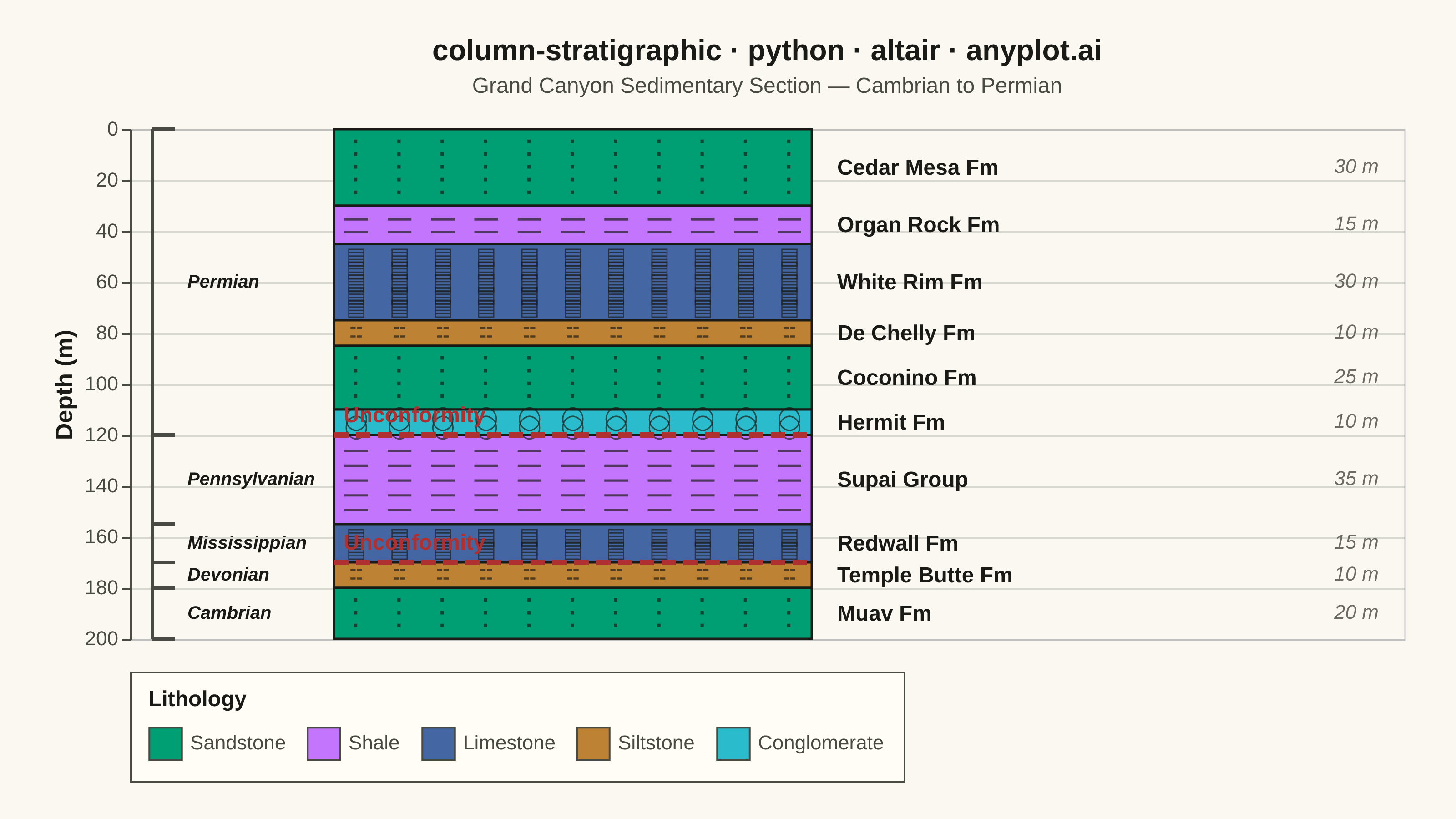
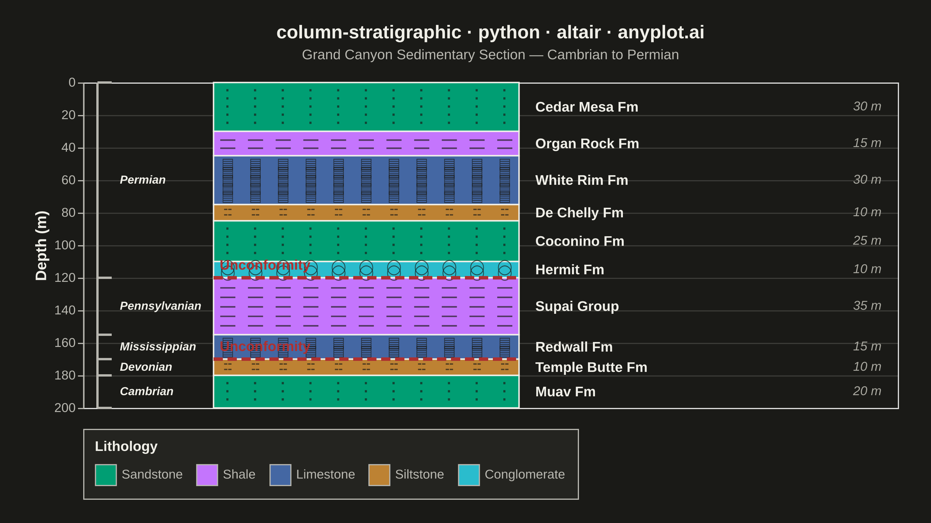
A vertical column visualization showing geological rock layers with standardized lithology patterns, formation names, ages, and thickness scales. Each layer is represented as a stacked rectangular block filled with a distinctive pattern (e.g., brick pattern for limestone, dots for sandstone, dashes for shale) following FGDC/USGS conventions. This plot is essential for communicating subsurface geology and sedimentary sequences in a compact, standardized format.
""" anyplot.ai
column-stratigraphic: Stratigraphic Column with Lithology Patterns
Library: altair 6.2.1 | Python 3.13.13
Quality: 87/100 | Updated: 2026-06-17
"""

import os

import altair as alt
import pandas as pd
from PIL import Image


# Theme-adaptive chrome (see prompts/default-style-guide.md "Theme-adaptive Chrome")
THEME = os.getenv("ANYPLOT_THEME", "light")
PAGE_BG = "#FAF8F1" if THEME == "light" else "#1A1A17"
ELEVATED_BG = "#FFFDF6" if THEME == "light" else "#242420"
INK = "#1A1A17" if THEME == "light" else "#F0EFE8"
INK_SOFT = "#4A4A44" if THEME == "light" else "#B8B7B0"
INK_MUTED = "#6B6A63" if THEME == "light" else "#A8A79F"

# Imprint palette — theme-independent categorical hues. Lithologies are abstract
# rock-type categories, so positions are assigned 1→N in canonical order, but
# position 5 (matte red #AE3030) is reserved as the semantic anchor for the
# unconformity markers (a gap/loss in the geological record) — so lithologies
# use positions 1,2,3,4,6.
LITHO_GREEN = "#009E73"  # Imprint 1 — brand, first categorical series
LITHO_LAV = "#C475FD"  # Imprint 2
LITHO_BLUE = "#4467A3"  # Imprint 3
LITHO_OCHRE = "#BD8233"  # Imprint 4
LITHO_CYAN = "#2ABCCD"  # Imprint 6
UNCONFORMITY = "#AE3030"  # Imprint 5 — semantic red for missing-time / unconformity

# Data: Grand Canyon sedimentary section, 10 layers spanning Cambrian to Permian
# Dramatic thickness variation (10-35 m) to showcase the stratigraphic format
layers = pd.DataFrame(
    {
        "top": [0, 30, 45, 75, 85, 110, 120, 155, 170, 180],
        "bottom": [30, 45, 75, 85, 110, 120, 155, 170, 180, 200],
        "lithology": [
            "Sandstone",
            "Shale",
            "Limestone",
            "Siltstone",
            "Sandstone",
            "Conglomerate",
            "Shale",
            "Limestone",
            "Siltstone",
            "Sandstone",
        ],
        "formation": [
            "Cedar Mesa Fm",
            "Organ Rock Fm",
            "White Rim Fm",
            "De Chelly Fm",
            "Coconino Fm",
            "Hermit Fm",
            "Supai Group",
            "Redwall Fm",
            "Temple Butte Fm",
            "Muav Fm",
        ],
        "age": [
            "Permian",
            "Permian",
            "Permian",
            "Permian",
            "Permian",
            "Permian",
            "Pennsylvanian",
            "Mississippian",
            "Devonian",
            "Cambrian",
        ],
    }
)

layers["thickness"] = layers["bottom"] - layers["top"]
layers["mid_depth"] = (layers["top"] + layers["bottom"]) / 2

# Lithology → Imprint palette (5 distinct rock types)
lithology_order = ["Sandstone", "Shale", "Limestone", "Siltstone", "Conglomerate"]
lithology_colors = {
    "Sandstone": LITHO_GREEN,
    "Shale": LITHO_LAV,
    "Limestone": LITHO_BLUE,
    "Siltstone": LITHO_OCHRE,
    "Conglomerate": LITHO_CYAN,
}

# Lithology pattern glyphs approximating FGDC/USGS texture conventions. Single
# motif per rock type, tiled across the full column width (rows × columns) so each
# layer reads as a true fill texture rather than a centered band.
pattern_symbols = {"Sandstone": "·", "Shale": "—", "Limestone": "▤", "Siltstone": "╌", "Conglomerate": "◯"}

# Column horizontal span (data units within x_domain) — the rectangles and the
# tiled texture share these bounds.
COL_L, COL_R = 3.2, 10.7

# Texture grid: tile each layer with rows (depth) × columns (across the width) of
# the lithology glyph, so the pattern fills the whole rectangle.
n_cols = 11
col_x = [COL_L + 0.35 + i * ((COL_R - COL_L - 0.7) / (n_cols - 1)) for i in range(n_cols)]
pattern_rows = []
for _, row in layers.iterrows():
    layer_height = row["bottom"] - row["top"]
    n_rows = max(2, int(layer_height / 6))
    spacing = layer_height / (n_rows + 1)
    sym = pattern_symbols[row["lithology"]]
    for i in range(n_rows):
        depth = row["top"] + spacing * (i + 1)
        for xp in col_x:
            pattern_rows.append({"depth": depth, "pattern": sym, "x_mid": xp})
pattern_df = pd.DataFrame(pattern_rows)

# Age groups — one bracket per contiguous geological period
age_groups = []
current_age = None
for _, row in layers.iterrows():
    if row["age"] != current_age:
        current_age = row["age"]
        group_rows = layers[layers["age"] == current_age]
        age_groups.append(
            {
                "age": current_age,
                "top": group_rows["top"].min(),
                "bottom": group_rows["bottom"].max(),
                "mid_depth": (group_rows["top"].min() + group_rows["bottom"].max()) / 2,
            }
        )
age_df = pd.DataFrame(age_groups)

# Unconformities at major age boundaries (missing time / erosional gaps)
unconformity_df = pd.DataFrame({"depth": [120, 170], "label": ["Unconformity", "Unconformity"]})

# Shared horizontal layout — generous x domain spreads side labels into clear lanes
x_domain = [0, 20]

# Layer rectangles — the stratigraphic column itself (x: 3.0 to 10.5)
rects = (
    alt.Chart(layers)
    .mark_rect(stroke=INK, strokeWidth=1.2)
    .encode(
        y=alt.Y(
            "top:Q",
            title="Depth (m)",
            scale=alt.Scale(domain=[0, 200], reverse=True),
            axis=alt.Axis(
                labelFontSize=11,
                titleFontSize=13,
                tickCount=10,
                gridColor=INK,
                gridOpacity=0.15,
                domainColor=INK_SOFT,
                domainWidth=1.2,
                tickColor=INK_SOFT,
                labelColor=INK_SOFT,
                titleColor=INK,
            ),
        ),
        y2="bottom:Q",
        x=alt.X("x:Q", scale=alt.Scale(domain=x_domain), axis=None),
        x2="x2:Q",
        color=alt.Color(
            "lithology:N",
            title="Lithology",
            scale=alt.Scale(domain=lithology_order, range=[lithology_colors[k] for k in lithology_order]),
            legend=alt.Legend(
                titleFontSize=12,
                labelFontSize=11,
                symbolSize=320,
                orient="bottom",
                titlePadding=8,
                direction="horizontal",
                labelLimit=200,
                symbolStrokeWidth=1.0,
                symbolStrokeColor=INK_SOFT,
                padding=10,
                columns=5,
            ),
        ),
        tooltip=[
            alt.Tooltip("formation:N", title="Formation"),
            alt.Tooltip("lithology:N", title="Lithology"),
            alt.Tooltip("age:N", title="Age"),
            alt.Tooltip("top:Q", title="Top (m)"),
            alt.Tooltip("bottom:Q", title="Bottom (m)"),
            alt.Tooltip("thickness:Q", title="Thickness (m)"),
        ],
    )
    .transform_calculate(x=f"{COL_L}", x2=f"{COL_R}")
)

# Tiled pattern texture overlay — dark ink reads on every Imprint fill in both themes
pattern_text = (
    alt.Chart(pattern_df)
    .mark_text(fontSize=13, color="#1A1A17", opacity=0.68, fontWeight="bold")
    .encode(y=alt.Y("depth:Q"), x=alt.X("x_mid:Q", scale=alt.Scale(domain=x_domain)), text="pattern:N")
)

# Formation name labels — to the right of the column
formation_labels = (
    alt.Chart(layers)
    .mark_text(fontSize=12, fontWeight="bold", align="left", color=INK)
    .encode(y=alt.Y("mid_depth:Q"), x=alt.X("x_pos:Q", scale=alt.Scale(domain=x_domain)), text="formation:N")
    .transform_calculate(x_pos=f"{COL_R + 0.4}")
)

# Thickness annotations — far-right lane, tertiary text
thickness_labels = (
    alt.Chart(layers)
    .mark_text(fontSize=11, align="right", color=INK_MUTED, fontStyle="italic")
    .encode(y=alt.Y("mid_depth:Q"), x=alt.X("x_pos:Q", scale=alt.Scale(domain=x_domain)), text="label:N")
    .transform_calculate(x_pos="19.6", label="datum.thickness + ' m'")
)

# Age bracket vertical lines — far-left, just clear of the depth-axis numerals
age_brackets_v = (
    alt.Chart(age_df)
    .mark_rule(strokeWidth=2.0, color=INK_SOFT)
    .encode(y=alt.Y("top:Q"), y2="bottom:Q", x=alt.X("x_pos:Q", scale=alt.Scale(domain=x_domain)))
    .transform_calculate(x_pos="0.35")
)

# Age period labels — left-aligned immediately right of the bracket so the long
# italic period names sit in their own lane between the bracket and the column,
# never reaching back into the depth-axis tick numbers (140/160/180).
age_labels = (
    alt.Chart(age_df)
    .mark_text(fontSize=10, fontStyle="italic", fontWeight="bold", align="left", color=INK)
    .encode(y=alt.Y("mid_depth:Q"), x=alt.X("x_pos:Q", scale=alt.Scale(domain=x_domain)), text="age:N")
    .transform_calculate(x_pos="0.9")
)

# Age bracket horizontal ticks (top and bottom of each age group)
bracket_ticks_data = []
for _, row in age_df.iterrows():
    bracket_ticks_data.append({"depth": row["top"]})
    bracket_ticks_data.append({"depth": row["bottom"]})
bracket_ticks_df = pd.DataFrame(bracket_ticks_data)

age_bracket_ticks = (
    alt.Chart(bracket_ticks_df)
    .mark_rule(strokeWidth=2.0, color=INK_SOFT)
    .encode(y=alt.Y("depth:Q"), x=alt.X("x1:Q", scale=alt.Scale(domain=x_domain)), x2="x2:Q")
    .transform_calculate(x1="0.35", x2="0.7")
)

# Unconformity markers — red dashed lines crossing the column at age boundaries
unconformity_rules = (
    alt.Chart(unconformity_df)
    .mark_rule(strokeWidth=3.0, color=UNCONFORMITY, strokeDash=[8, 4])
    .encode(y=alt.Y("depth:Q"), x=alt.X("x1:Q", scale=alt.Scale(domain=x_domain)), x2="x2:Q")
    .transform_calculate(x1=f"{COL_L}", x2=f"{COL_R}")
)

# Unconformity labels — pinned just inside the column's left edge, lifted clear of
# the layer texture above the dashed rule
unconformity_labels_chart = (
    alt.Chart(unconformity_df)
    .mark_text(fontSize=12, color=UNCONFORMITY, fontWeight="bold", align="left", dy=-11)
    .encode(y=alt.Y("depth:Q"), x=alt.X("x_pos:Q", scale=alt.Scale(domain=x_domain)), text="label:N")
    .transform_calculate(x_pos=f"{COL_L + 0.15}")
)

# Compose all layers
title = "column-stratigraphic · python · altair · anyplot.ai"
chart = (
    (
        rects
        + pattern_text
        + formation_labels
        + thickness_labels
        + age_labels
        + age_brackets_v
        + age_bracket_ticks
        + unconformity_rules
        + unconformity_labels_chart
    )
    .properties(
        width=700,
        height=280,
        title=alt.Title(
            title,
            fontSize=16,
            anchor="middle",
            offset=12,
            color=INK,
            subtitle="Grand Canyon Sedimentary Section — Cambrian to Permian",
            subtitleFontSize=12,
            subtitleColor=INK_SOFT,
            subtitlePadding=6,
        ),
    )
    .configure_view(strokeWidth=0, fill=PAGE_BG)
    .configure(background=PAGE_BG)
    .configure_legend(fillColor=ELEVATED_BG, strokeColor=INK_SOFT, labelColor=INK_SOFT, titleColor=INK)
)

# Save PNG, then PAD-only up to the exact landscape target (never crop — see altair.md)
chart.save(f"plot-{THEME}.png", scale_factor=4.0)

TW, TH = 3200, 1800
_img = Image.open(f"plot-{THEME}.png").convert("RGB")
_w, _h = _img.size
if _w > TW or _h > TH:
    raise SystemExit(
        f"altair vl-convert produced {_w}×{_h}, exceeds target {TW}×{TH}. "
        f"Shrink chart .properties(width=, height=) values and re-render."
    )
if _w < TW or _h < TH:
    _canvas = Image.new("RGB", (TW, TH), PAGE_BG)
    _canvas.paste(_img, ((TW - _w) // 2, (TH - _h) // 2))
    _canvas.save(f"plot-{THEME}.png")

chart.save(f"plot-{THEME}.html")
Runnable source as JSON, for any HTTP client: https://api.anyplot.ai/specs/column-stratigraphic/altair/code. Any spec id and library id listed in llms-full.txt fit the same URL shape; every URL below is complete and callable.
{
  "spec_id": "column-stratigraphic",
  "language": "python",
  "library": "altair",
  "page": "https://anyplot.ai/column-stratigraphic/python/altair",
  "hub": "https://anyplot.ai/column-stratigraphic",
  "code_json": "https://api.anyplot.ai/specs/column-stratigraphic/altair/code",
  "spec_json": "https://api.anyplot.ai/specs/column-stratigraphic",
  "render_light_png": "https://storage.googleapis.com/anyplot-images/plots/column-stratigraphic/python/altair/plot-light.png",
  "render_dark_png": "https://storage.googleapis.com/anyplot-images/plots/column-stratigraphic/python/altair/plot-dark.png",
  "interactive_light_html": "https://storage.googleapis.com/anyplot-images/plots/column-stratigraphic/python/altair/plot-light.html",
  "interactive_dark_html": "https://storage.googleapis.com/anyplot-images/plots/column-stratigraphic/python/altair/plot-dark.html",
  "quality_score": 87.0,
  "license": "MIT",
  "guide": "https://anyplot.ai/llms.txt"
}
Part of Stratigraphic Column with Lithology Patterns on anyplot.ai.