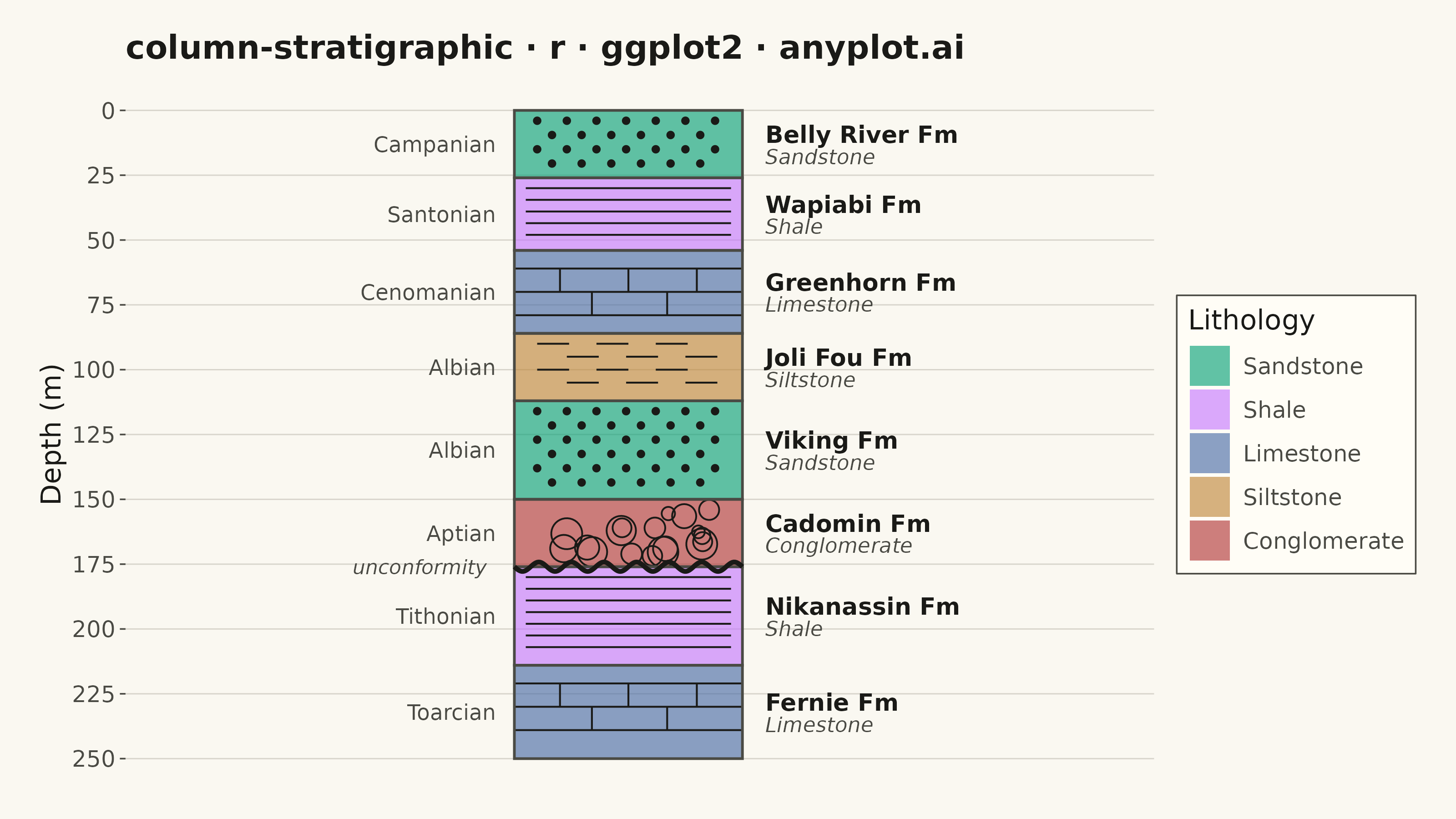
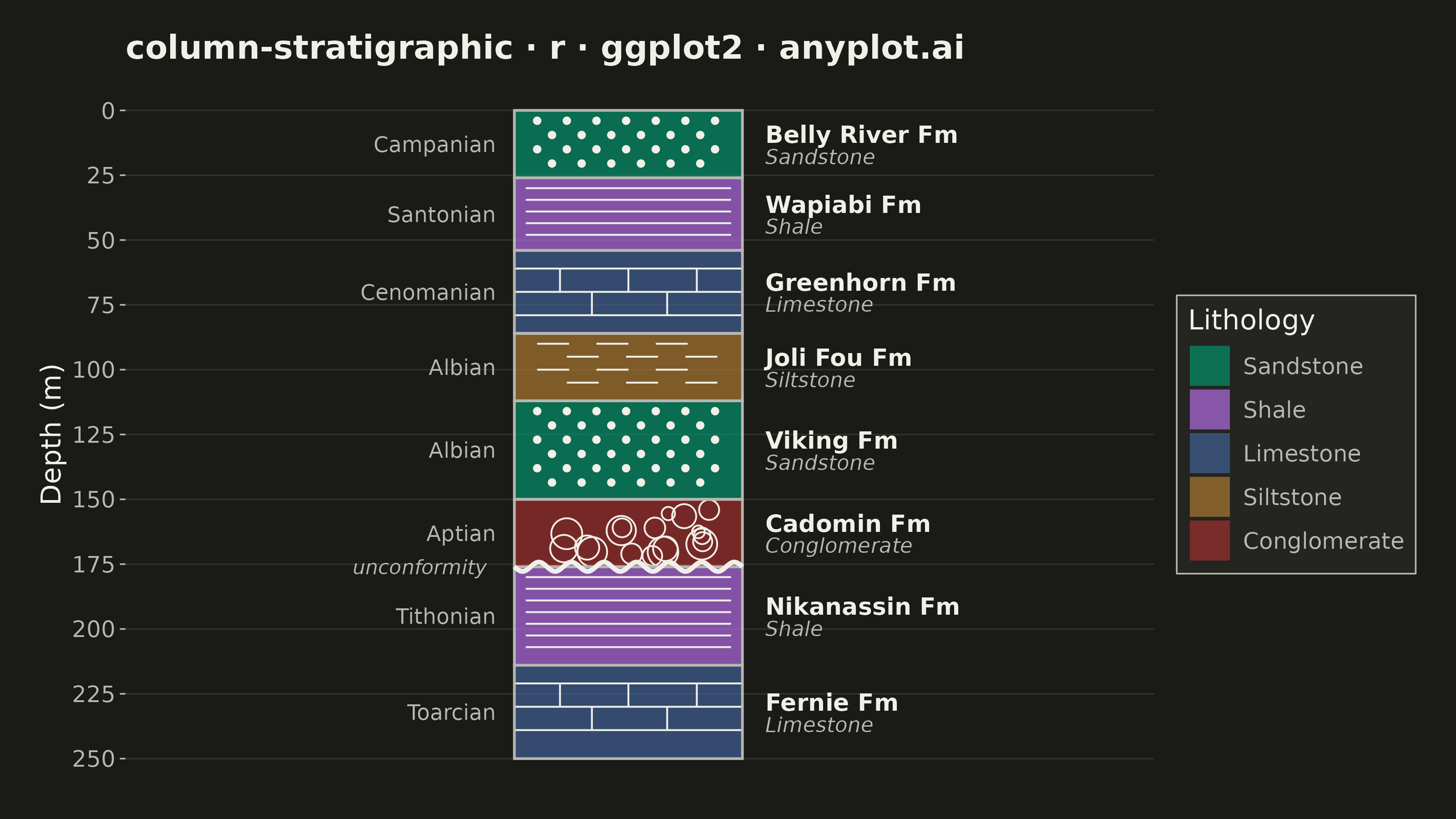
A vertical column visualization showing geological rock layers with standardized lithology patterns, formation names, ages, and thickness scales. Each layer is represented as a stacked rectangular block filled with a distinctive pattern (e.g., brick pattern for limestone, dots for sandstone, dashes for shale) following FGDC/USGS conventions. This plot is essential for communicating subsurface geology and sedimentary sequences in a compact, standardized format.
#' anyplot.ai
#' column-stratigraphic: Stratigraphic Column with Lithology Patterns
#' Library: ggplot2 3.5.1 | R 4.4.1
#' Quality: 93/100 | Created: 2026-06-17

library(ggplot2)
library(dplyr)
library(tibble)
library(ragg)

set.seed(42)

# --- Theme tokens -----------------------------------------------------------
THEME       <- Sys.getenv("ANYPLOT_THEME", "light")
PAGE_BG     <- if (THEME == "light") "#FAF8F1" else "#1A1A17"
ELEVATED_BG <- if (THEME == "light") "#FFFDF6" else "#242420"
INK         <- if (THEME == "light") "#1A1A17" else "#F0EFE8"
INK_SOFT    <- if (THEME == "light") "#4A4A44" else "#B8B7B0"
GRID        <- if (THEME == "light") "#D8D5CC" else "#33332E"

# Imprint palette — canonical order, first series ALWAYS #009E73.
# Lithology is encoded primarily by the FGDC/USGS-style fill pattern; the colour
# is a secondary tint, so the categories take the Imprint palette in order.
LITH_COLORS <- c(
  Sandstone    = "#009E73",  # 1 — brand green (first series)
  Shale        = "#C475FD",  # 2 — lavender
  Limestone    = "#4467A3",  # 3 — blue
  Siltstone    = "#BD8233",  # 4 — ochre
  Conglomerate = "#AE3030"   # 5 — matte red
)

# --- Data: a synthetic borehole section (depth increases downward) ----------
layers <- tibble(
  top       = c(0,   26,  54,  86,  112, 150, 176, 214),
  bottom    = c(26,  54,  86,  112, 150, 176, 214, 250),
  lithology = c("Sandstone", "Shale", "Limestone", "Siltstone",
                "Sandstone", "Conglomerate", "Shale", "Limestone"),
  formation = c("Belly River Fm", "Wapiabi Fm", "Greenhorn Fm", "Joli Fou Fm",
                "Viking Fm", "Cadomin Fm", "Nikanassin Fm", "Fernie Fm"),
  age       = c("Campanian", "Santonian", "Cenomanian", "Albian",
                "Albian", "Aptian", "Tithonian", "Toarcian")
)
layers$lithology <- factor(layers$lithology, levels = names(LITH_COLORS))

# A sub-Cretaceous unconformity (Aptian conglomerate over Tithonian shale).
UNCONFORMITY <- 176

# --- Build the lithology patterns natively (line / dot / clast primitives) ---
# ggplot2 has no native fill-texture geom, so each rock type's standard symbol
# is composed from segments, points and open circles laid inside the layer box.
seg_rows <- list(); dot_rows <- list(); clast_rows <- list()
si <- 0L; di <- 0L; ci <- 0L

for (i in seq_len(nrow(layers))) {
    t <- layers$top[i]; b <- layers$bottom[i]
    lit <- as.character(layers$lithology[i])

    if (lit == "Limestone") {
        # Brick: full-width courses with staggered vertical joints.
        courses <- seq(t + 7, b - 3, by = 9)
        si <- si + 1L
        seg_rows[[si]] <- tibble(x = 0.0, xend = 1.0, y = courses, yend = courses)
        if (length(courses) >= 2) {
            for (j in seq_len(length(courses) - 1)) {
                xv <- if (j %% 2 == 0) c(0.34, 0.67) else c(0.2, 0.5, 0.8)
                si <- si + 1L
                seg_rows[[si]] <- tibble(x = xv, xend = xv,
                                         y = courses[j], yend = courses[j + 1])
            }
        }
    } else if (lit == "Shale") {
        # Continuous, closely spaced horizontal laminae.
        lines_y <- seq(t + 4, b - 3, by = 4.5)
        si <- si + 1L
        seg_rows[[si]] <- tibble(x = 0.05, xend = 0.95, y = lines_y, yend = lines_y)
    } else if (lit == "Siltstone") {
        # Broken (dashed) horizontal lines, staggered between rows.
        rows <- seq(t + 4, b - 3, by = 5)
        for (j in seq_along(rows)) {
            xo <- if (j %% 2 == 0) 0.13 else 0
            xs <- seq(0.1 + xo, 0.82, by = 0.26)
            si <- si + 1L
            seg_rows[[si]] <- tibble(x = xs, xend = xs + 0.14,
                                     y = rows[j], yend = rows[j])
        }
    } else if (lit == "Sandstone") {
        # Stipple: regular dot grid, offset on alternate rows.
        rows <- seq(t + 4, b - 3, by = 5.5)
        for (j in seq_along(rows)) {
            xo <- if (j %% 2 == 0) 0.065 else 0
            xs <- seq(0.1 + xo, 0.93, by = 0.13)
            di <- di + 1L
            dot_rows[[di]] <- tibble(x = xs, y = rep(rows[j], length(xs)))
        }
    } else if (lit == "Conglomerate") {
        # Scattered clasts as open circles of varying size.
        n <- max(8L, round((b - t) * 0.7))
        ci <- ci + 1L
        clast_rows[[ci]] <- tibble(
            x = runif(n, 0.13, 0.87),
            y = runif(n, t + 4, b - 4),
            r = runif(n, 2.0, 5.5)
        )
    }
}
seg_df   <- bind_rows(seg_rows)
dot_df   <- bind_rows(dot_rows)
clast_df <- bind_rows(clast_rows)

# Wavy line marking the unconformity contact.
wave <- tibble(x = seq(0, 1, length.out = 160))
wave$y <- UNCONFORMITY + 1.8 * sin(wave$x * 2 * pi * 7)

# --- Plot -------------------------------------------------------------------
p <- ggplot() +
    geom_rect(data = layers,
              aes(xmin = 0, xmax = 1, ymin = top, ymax = bottom, fill = lithology),
              color = NA, alpha = 0.62) +
    geom_segment(data = seg_df, aes(x = x, xend = xend, y = y, yend = yend),
                 color = INK, linewidth = 0.35) +
    geom_point(data = dot_df, aes(x = x, y = y), color = INK, size = 0.9) +
    geom_point(data = clast_df, aes(x = x, y = y, size = r),
               shape = 1, stroke = 0.5, color = INK) +
    scale_size_identity() +
    geom_rect(data = layers,
              aes(xmin = 0, xmax = 1, ymin = top, ymax = bottom),
              fill = NA, color = INK_SOFT, linewidth = 0.5) +
    geom_path(data = wave, aes(x = x, y = y), color = INK, linewidth = 0.9) +
    annotate("text", x = -0.12, y = UNCONFORMITY, label = "unconformity",
             hjust = 1, fontface = "italic", size = 2.8, color = INK_SOFT) +
    geom_text(data = layers,
              aes(x = 1.1, y = (top + bottom) / 2 - 3.8, label = formation),
              hjust = 0, fontface = "bold", size = 3.3, color = INK) +
    geom_text(data = layers,
              aes(x = 1.1, y = (top + bottom) / 2 + 4.8, label = lithology),
              hjust = 0, fontface = "italic", size = 2.9, color = INK_SOFT) +
    geom_text(data = layers,
              aes(x = -0.08, y = (top + bottom) / 2, label = age),
              hjust = 1, size = 3.0, color = INK_SOFT) +
    scale_fill_manual(values = LITH_COLORS, name = "Lithology",
                      breaks = names(LITH_COLORS)) +
    scale_y_reverse(breaks = seq(0, 250, 25),
                    expand = expansion(mult = c(0.03, 0.03))) +
    coord_cartesian(xlim = c(-1.5, 2.6), clip = "off") +
    guides(fill = guide_legend(override.aes = list(alpha = 0.62))) +
    labs(title = "column-stratigraphic · r · ggplot2 · anyplot.ai",
         y = "Depth (m)", x = NULL) +
    theme_minimal(base_size = 9) +
    theme(
        plot.background    = element_rect(fill = PAGE_BG, color = PAGE_BG),
        panel.background   = element_rect(fill = PAGE_BG, color = NA),
        panel.grid         = element_blank(),
        panel.grid.major.y = element_line(color = GRID, linewidth = 0.25),
        axis.title.y       = element_text(color = INK, size = 11),
        axis.text.y        = element_text(color = INK_SOFT, size = 9),
        axis.title.x       = element_blank(),
        axis.text.x        = element_blank(),
        axis.ticks.x       = element_blank(),
        axis.ticks.y       = element_line(color = INK_SOFT, linewidth = 0.3),
        plot.title         = element_text(color = INK, size = 13, face = "bold",
                                          margin = margin(b = 10)),
        legend.position    = "right",
        legend.title       = element_text(color = INK, size = 11),
        legend.text        = element_text(color = INK_SOFT, size = 9),
        legend.background   = element_rect(fill = ELEVATED_BG, color = INK_SOFT,
                                          linewidth = 0.3),
        legend.key         = element_rect(fill = ELEVATED_BG, color = NA),
        plot.margin        = margin(t = 14, r = 16, b = 14, l = 16)
    )

# --- Save -------------------------------------------------------------------
ggsave(
    filename = sprintf("plot-%s.png", THEME),
    plot     = p,
    device   = ragg::agg_png,
    width    = 8,
    height   = 4.5,
    units    = "in",
    dpi      = 400
)
Runnable source as JSON, for any HTTP client: https://api.anyplot.ai/specs/column-stratigraphic/ggplot2/code. Any spec id and library id listed in llms-full.txt fit the same URL shape; every URL below is complete and callable.
{
  "spec_id": "column-stratigraphic",
  "language": "r",
  "library": "ggplot2",
  "page": "https://anyplot.ai/column-stratigraphic/r/ggplot2",
  "hub": "https://anyplot.ai/column-stratigraphic",
  "code_json": "https://api.anyplot.ai/specs/column-stratigraphic/ggplot2/code",
  "spec_json": "https://api.anyplot.ai/specs/column-stratigraphic",
  "render_light_png": "https://storage.googleapis.com/anyplot-images/plots/column-stratigraphic/r/ggplot2/plot-light.png",
  "render_dark_png": "https://storage.googleapis.com/anyplot-images/plots/column-stratigraphic/r/ggplot2/plot-dark.png",
  "quality_score": 93.0,
  "license": "MIT",
  "guide": "https://anyplot.ai/llms.txt"
}
Part of Stratigraphic Column with Lithology Patterns on anyplot.ai.