The same plot in 14 other libraries — JavaScript: Chart.js, D3.js, Apache ECharts, Highcharts; Python: Altair, Bokeh, lets-plot, Matplotlib, Plotly, plotnine, Pygal, Seaborn; R: ggplot2; Julia: Makie.jl. Compare all 15 side by side: Decision Boundary Classifier Visualization in Python, R, Julia and JavaScript.
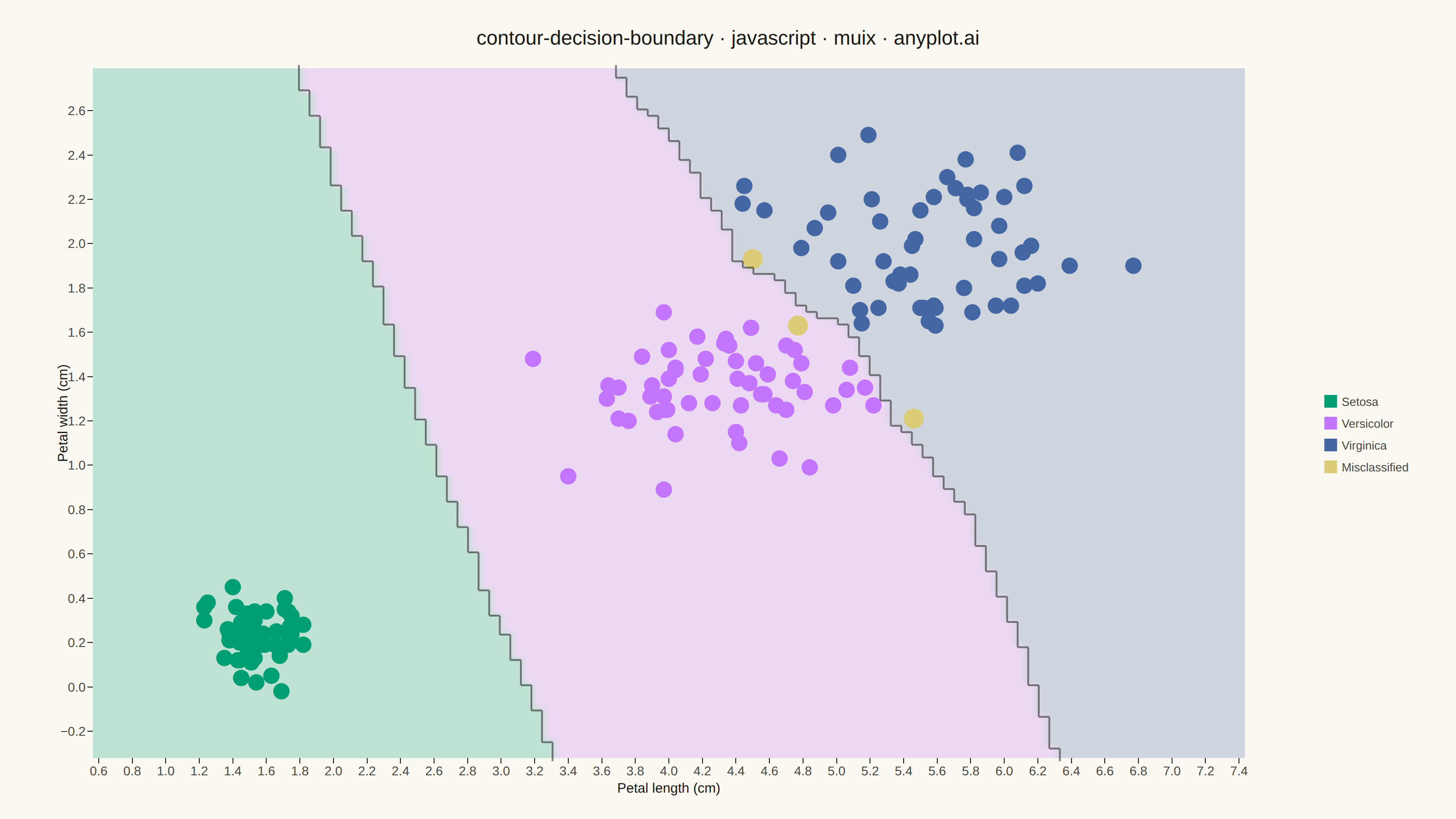
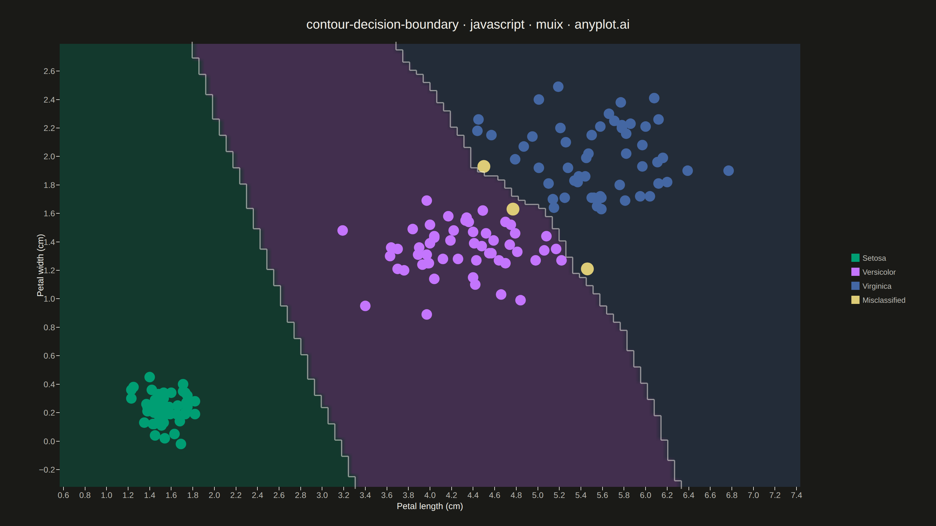
A decision boundary visualization showing how a classifier partitions 2D feature space into predicted class regions. Colored regions indicate the predicted class at each point in the feature space, with training data points overlaid to show how well the classifier separates different classes. This visualization is essential for understanding classifier behavior, identifying decision boundaries, and evaluating classification accuracy in machine learning.
// anyplot.ai
// contour-decision-boundary: Decision Boundary Classifier Visualization
// Library: muix 7.29.1 | JavaScript 22.23.2
// Quality: 87/100 | Created: 2026-09-04

import { ScatterChart } from "@mui/x-charts/ScatterChart";
import { useDrawingArea } from "@mui/x-charts/hooks";
import Box from "@mui/material/Box";
import Typography from "@mui/material/Typography";

const t = window.ANYPLOT_TOKENS;

// Deterministic LCG (seed 42) — no Math.random() in the browser harness
function makeLcg(seed) {
  let state = seed >>> 0;
  return () => {
    state = (Math.imul(state, 1664525) + 1013904223) >>> 0;
    return state / 4294967296;
  };
}
const rng = makeLcg(42);

// Box-Muller standard normal draw, fed by the LCG above.
function gaussian() {
  const u1 = Math.max(rng(), 1e-9);
  const u2 = rng();
  return Math.sqrt(-2 * Math.log(u1)) * Math.cos(2 * Math.PI * u2);
}

// --- Data: synthetic iris-like petal measurements, 3 species ---------------
// Setosa is fully separable on these two features; versicolor and virginica
// overlap near the boundary — the same pattern the real iris dataset shows,
// which is what makes a few training points fall on the wrong side.
const SPECIES = [
  { name: "Setosa", meanX: 1.5, meanY: 0.25, stdX: 0.17, stdY: 0.1, n: 50 },
  { name: "Versicolor", meanX: 4.3, meanY: 1.3, stdX: 0.47, stdY: 0.2, n: 55 },
  { name: "Virginica", meanX: 5.55, meanY: 2.03, stdX: 0.55, stdY: 0.27, n: 55 },
];

let pointId = 0;
const trainingPoints = SPECIES.flatMap((sp, cls) =>
  Array.from({ length: sp.n }, () => ({
    id: `iris-${pointId++}`,
    x: Math.round((sp.meanX + gaussian() * sp.stdX) * 100) / 100,
    y: Math.round((sp.meanY + gaussian() * sp.stdY) * 100) / 100,
    cls,
  })),
);

// --- k-nearest-neighbors classifier (k=13, squared distance, majority vote) -
// k=13 (vs. a smaller k) widens each point's neighborhood just enough to pull
// in 2-3 genuine misclassifications near different spots along the
// Versicolor/Virginica boundary, instead of only one.
const K = 13;
function knnPredict(px, py, excludeId) {
  const neighbors = [];
  for (const p of trainingPoints) {
    if (p.id === excludeId) continue;
    const dx = px - p.x;
    const dy = py - p.y;
    neighbors.push({ d2: dx * dx + dy * dy, cls: p.cls });
  }
  neighbors.sort((a, b) => a.d2 - b.d2);
  const votes = new Map();
  for (let i = 0; i < K && i < neighbors.length; i += 1) {
    votes.set(neighbors[i].cls, (votes.get(neighbors[i].cls) || 0) + 1);
  }
  let bestCls = 0;
  let bestVotes = -1;
  votes.forEach((count, cls) => {
    if (count > bestVotes) {
      bestVotes = count;
      bestCls = cls;
    }
  });
  return bestCls;
}

// Leave-one-out prediction — predicting a point against a set that includes
// itself would trivially match, hiding real misclassifications.
trainingPoints.forEach((p) => {
  p.predicted = knnPredict(p.x, p.y, p.id);
  p.correct = p.predicted === p.cls;
});

// --- Dense mesh grid: classifier prediction at every cell -------------------
const GRID = 110;
const trainX = trainingPoints.map((p) => p.x);
const trainY = trainingPoints.map((p) => p.y);
const padX = (Math.max(...trainX) - Math.min(...trainX)) * 0.12;
const padY = (Math.max(...trainY) - Math.min(...trainY)) * 0.12;
const X_MIN = Math.min(...trainX) - padX;
const X_MAX = Math.max(...trainX) + padX;
const Y_MIN = Math.min(...trainY) - padY;
const Y_MAX = Math.max(...trainY) + padY;

const xs = Array.from({ length: GRID }, (_, i) => X_MIN + (i / (GRID - 1)) * (X_MAX - X_MIN));
const ys = Array.from({ length: GRID }, (_, j) => Y_MIN + (j / (GRID - 1)) * (Y_MAX - Y_MIN));
const classGrid = ys.map((y) => xs.map((x) => knnPredict(x, y)));

// --- Region fill: rasterize the classifier's predicted class at every mesh
// cell into an off-screen canvas, one pixel per cell, then stretch it under
// the chart as a plain <img>. This paints a genuinely smooth, contiguous
// region fill straight from the real grid predictions (no fake data) instead
// of thousands of overlapping scatter markers, which read as a stippled dot
// texture rather than a deliberate area fill.
const CLASS_COLORS = [t.palette[0], t.palette[1], t.palette[2]];
const REGION_ALPHA = 0.24;

function hexToRgb(hex) {
  return [parseInt(hex.slice(1, 3), 16), parseInt(hex.slice(3, 5), 16), parseInt(hex.slice(5, 7), 16)];
}
const classRgb = CLASS_COLORS.map(hexToRgb);

function buildRegionFillDataUrl() {
  const canvas = document.createElement("canvas");
  canvas.width = GRID;
  canvas.height = GRID;
  const ctx = canvas.getContext("2d");
  const imageData = ctx.createImageData(GRID, GRID);
  ys.forEach((_y, j) => {
    // Canvas row 0 is the top of the image; ys[0] is Y_MIN (the bottom of the
    // plot), so row = GRID - 1 - j flips the mesh into image space.
    const row = GRID - 1 - j;
    xs.forEach((_x, i) => {
      const [r, g, b] = classRgb[classGrid[j][i]];
      const idx = (row * GRID + i) * 4;
      imageData.data[idx] = r;
      imageData.data[idx + 1] = g;
      imageData.data[idx + 2] = b;
      imageData.data[idx + 3] = Math.round(REGION_ALPHA * 255);
    });
  });
  ctx.putImageData(imageData, 0, 0);
  return canvas.toDataURL();
}
const regionFillDataUrl = buildRegionFillDataUrl();

// --- Boundary trace: a staircase along the mesh cells where the predicted
// class changes between neighbours — the actual decision boundary read off
// the grid, not a fitted curve.
function boundarySegments() {
  const halfDx = (xs[1] - xs[0]) / 2;
  const halfDy = (ys[1] - ys[0]) / 2;
  const segs = [];
  for (let j = 0; j < GRID; j += 1) {
    for (let i = 0; i < GRID - 1; i += 1) {
      if (classGrid[j][i] !== classGrid[j][i + 1]) {
        const xm = (xs[i] + xs[i + 1]) / 2;
        segs.push([
          [xm, ys[j] - halfDy],
          [xm, ys[j] + halfDy],
        ]);
      }
    }
  }
  for (let j = 0; j < GRID - 1; j += 1) {
    for (let i = 0; i < GRID; i += 1) {
      if (classGrid[j][i] !== classGrid[j + 1][i]) {
        const ym = (ys[j] + ys[j + 1]) / 2;
        segs.push([
          [xs[i] - halfDx, ym],
          [xs[i] + halfDx, ym],
        ]);
      }
    }
  }
  return segs;
}
const boundary = boundarySegments();

// --- SVG boundary overlay (rendered as a ScatterChart child) ---------------
function BoundaryOverlay() {
  const { left, top, width, height } = useDrawingArea();
  const toSVG = (dx, dy) => [
    left + ((dx - X_MIN) / (X_MAX - X_MIN)) * width,
    top + (1 - (dy - Y_MIN) / (Y_MAX - Y_MIN)) * height,
  ];
  const d = boundary
    .map(([p0, p1]) => {
      const [x0, y0] = toSVG(p0[0], p0[1]);
      const [x1, y1] = toSVG(p1[0], p1[1]);
      return `M ${x0.toFixed(1)},${y0.toFixed(1)} L ${x1.toFixed(1)},${y1.toFixed(1)}`;
    })
    .join(" ");
  return <path d={d} stroke={t.ink} strokeWidth={2} strokeOpacity={0.55} fill="none" />;
}

// --- Training-point overlay --------------------------------------------------
// Correctly classified points keep their species color; misclassified points
// switch to the amber warning anchor so the classifier's mistakes stand out
// against the region fill.
const correctSeries = SPECIES.map((sp, cls) => ({
  id: `species-${cls}`,
  label: sp.name,
  data: trainingPoints
    .filter((p) => p.cls === cls && p.correct)
    .map((p) => ({ x: p.x, y: p.y, id: p.id })),
  color: CLASS_COLORS[cls],
  markerSize: 9,
}));

const misclassifiedSeries = {
  id: "misclassified",
  label: "Misclassified",
  data: trainingPoints
    .filter((p) => !p.correct)
    .map((p) => ({ x: p.x, y: p.y, id: p.id })),
  color: t.amber,
  markerSize: 11,
};

const TITLE = "contour-decision-boundary · javascript · muix · anyplot.ai";

// Fixed pixel margin, shared by the ScatterChart's own `margin` prop and the
// region-fill <img> below — both need to agree on exactly where the drawing
// area starts.
const MARGIN = { left: 70, right: 200, top: 12, bottom: 58 };

// --- Chart (default-exported component — the harness mounts it) -----------
export default function Chart() {
  const W = window.ANYPLOT_SIZE.width;
  const H = window.ANYPLOT_SIZE.height;
  const chartW = W - 64;
  const chartH = H - 28 - 36 - 8;
  const drawW = chartW - MARGIN.left - MARGIN.right;
  const drawH = chartH - MARGIN.top - MARGIN.bottom;
  return (
    <Box
      sx={{
        width: W,
        height: H,
        display: "flex",
        flexDirection: "column",
        bgcolor: t.pageBg,
        boxSizing: "border-box",
        pt: "28px",
        px: "32px",
        pb: "8px",
      }}
    >
      <Typography
        component="div"
        sx={{ fontSize: 22, fontWeight: 500, color: t.ink, textAlign: "center", lineHeight: 1.3, mb: "6px", flexShrink: 0 }}
      >
        {TITLE}
      </Typography>
      <Box sx={{ position: "relative", width: chartW, height: chartH, flexShrink: 0 }}>
        {/* Region-fill wash sits behind the chart; the ScatterChart itself stays
            transparent so its dots and boundary line render crisply on top. */}
        <Box
          component="img"
          src={regionFillDataUrl}
          alt=""
          sx={{ position: "absolute", left: MARGIN.left, top: MARGIN.top, width: drawW, height: drawH, pointerEvents: "none" }}
        />
        <ScatterChart
          width={chartW}
          height={chartH}
          skipAnimation
          tooltip={{ trigger: "none" }}
          series={[...correctSeries, misclassifiedSeries]}
          xAxis={[
            {
              min: X_MIN,
              max: X_MAX,
              label: "Petal length (cm)",
              disableLine: true,
              labelStyle: { fontSize: 15, fill: t.ink },
              tickLabelStyle: { fontSize: 14, fill: t.inkSoft },
            },
          ]}
          yAxis={[
            {
              min: Y_MIN,
              max: Y_MAX,
              label: "Petal width (cm)",
              disableLine: true,
              labelStyle: { fontSize: 15, fill: t.ink },
              tickLabelStyle: { fontSize: 14, fill: t.inkSoft },
            },
          ]}
          margin={MARGIN}
          sx={{ position: "relative" }}
          slotProps={{
            legend: {
              direction: "column",
              position: { vertical: "middle", horizontal: "right" },
              itemMarkWidth: 14,
              itemMarkHeight: 14,
              labelStyle: { fontSize: 13, fill: t.inkSoft },
            },
          }}
        >
          <BoundaryOverlay />
        </ScatterChart>
      </Box>
    </Box>
  );
}
Runnable source as JSON, for any HTTP client: https://api.anyplot.ai/specs/contour-decision-boundary/muix/code. Any spec id and library id listed in llms-full.txt fit the same URL shape; every URL below is complete and callable.
{
  "spec_id": "contour-decision-boundary",
  "language": "javascript",
  "library": "muix",
  "page": "https://anyplot.ai/contour-decision-boundary/javascript/muix",
  "hub": "https://anyplot.ai/contour-decision-boundary",
  "code_json": "https://api.anyplot.ai/specs/contour-decision-boundary/muix/code",
  "spec_json": "https://api.anyplot.ai/specs/contour-decision-boundary",
  "render_light_png": "https://storage.googleapis.com/anyplot-images/plots/contour-decision-boundary/javascript/muix/plot-light.png",
  "render_dark_png": "https://storage.googleapis.com/anyplot-images/plots/contour-decision-boundary/javascript/muix/plot-dark.png",
  "interactive_light_html": "https://storage.googleapis.com/anyplot-images/plots/contour-decision-boundary/javascript/muix/plot-light.html",
  "interactive_dark_html": "https://storage.googleapis.com/anyplot-images/plots/contour-decision-boundary/javascript/muix/plot-dark.html",
  "quality_score": 87.0,
  "license": "MIT",
  "guide": "https://anyplot.ai/llms.txt"
}
Part of Decision Boundary Classifier Visualization on anyplot.ai.