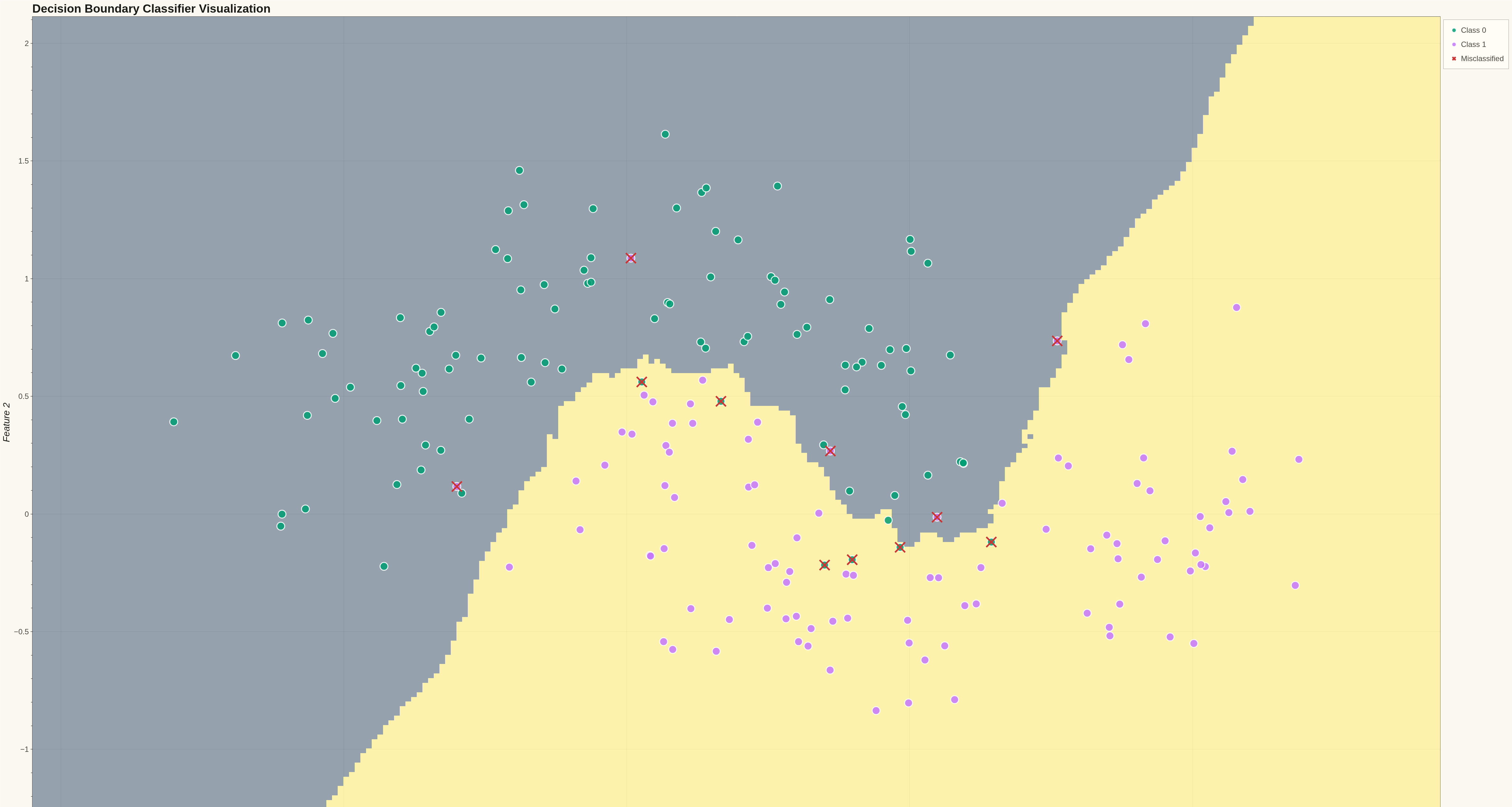
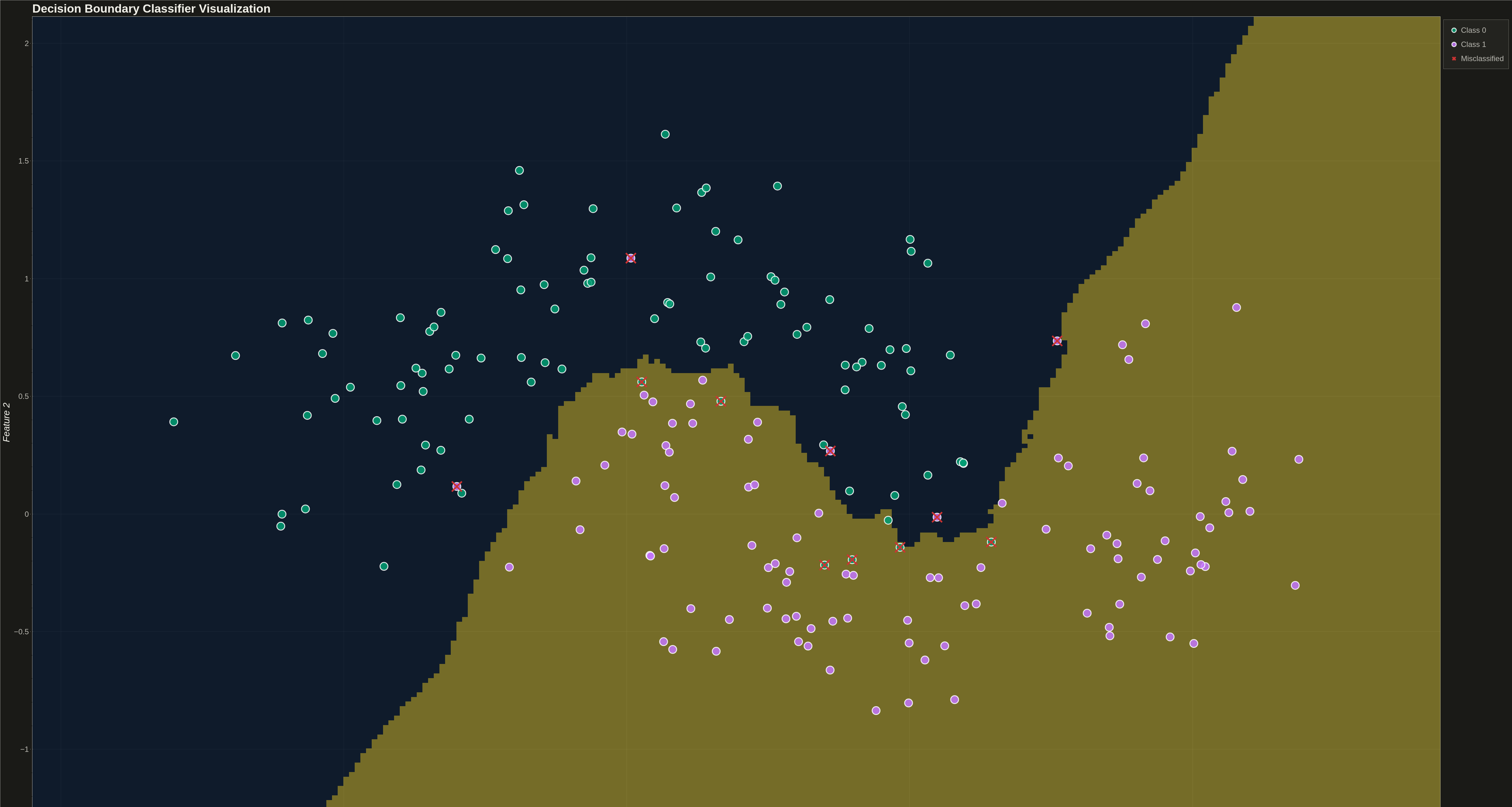
A decision boundary visualization showing how a classifier partitions 2D feature space into predicted class regions. Colored regions indicate the predicted class at each point in the feature space, with training data points overlaid to show how well the classifier separates different classes. This visualization is essential for understanding classifier behavior, identifying decision boundaries, and evaluating classification accuracy in machine learning.
""" anyplot.ai
contour-decision-boundary: Decision Boundary Classifier Visualization
Library: bokeh 3.9.0 | Python 3.13.13
Quality: 85/100 | Updated: 2026-05-16
"""

import os
import sys
import time
from pathlib import Path


# Remove current directory from path to avoid shadowing bokeh package
if "" in sys.path:
    sys.path.remove("")
sys.path.insert(0, "/home/runner/work/anyplot/anyplot/.venv/lib/python3.13/site-packages")

# Change to script directory to save files in the correct location
os.chdir(os.path.dirname(os.path.abspath(__file__)))

# isort: off
import numpy as np
from bokeh.io import output_file, save
from bokeh.models import (
    ColumnDataSource,
    HoverTool,
    Legend,
    LegendItem,
    LinearColorMapper,
)
from bokeh.palettes import Cividis256
from bokeh.plotting import figure
from selenium import webdriver
from selenium.webdriver.chrome.options import Options
from sklearn.datasets import make_moons
from sklearn.neighbors import KNeighborsClassifier
# isort: on

# Theme tokens
THEME = os.getenv("ANYPLOT_THEME", "light")
PAGE_BG = "#FAF8F1" if THEME == "light" else "#1A1A17"
ELEVATED_BG = "#FFFDF6" if THEME == "light" else "#242420"
INK = "#1A1A17" if THEME == "light" else "#F0EFE8"
INK_SOFT = "#4A4A44" if THEME == "light" else "#B8B7B0"

# Okabe-Ito colors for classes
CLASS_COLORS = ["#009E73", "#C475FD"]  # Positions 1 and 2 of the palette

# Data - Generate synthetic classification data
np.random.seed(42)
X, y = make_moons(n_samples=200, noise=0.25, random_state=42)

# Train a classifier
clf = KNeighborsClassifier(n_neighbors=15)
clf.fit(X, y)

# Create mesh grid for decision boundary
x_min, x_max = X[:, 0].min() - 0.5, X[:, 0].max() + 0.5
y_min, y_max = X[:, 1].min() - 0.5, X[:, 1].max() + 0.5
h = 0.02  # Step size
xx, yy = np.meshgrid(np.arange(x_min, x_max, h), np.arange(y_min, y_max, h))

# Get predictions for mesh grid
Z = clf.predict(np.c_[xx.ravel(), yy.ravel()])
Z = Z.reshape(xx.shape)

# Create figure
p = figure(
    width=4800,
    height=2700,
    title="Decision Boundary Classifier Visualization",
    x_axis_label="Feature 1",
    y_axis_label="Feature 2",
    tools="",
    toolbar_location=None,
    x_range=(x_min, x_max),
    y_range=(y_min, y_max),
)

# Use continuous colormap for decision regions (Cividis for diverging appearance)
color_mapper = LinearColorMapper(palette=Cividis256, low=0, high=1)
p.image(
    image=[Z.astype(float)], x=x_min, y=y_min, dw=x_max - x_min, dh=y_max - y_min, color_mapper=color_mapper, alpha=0.4
)

# Separate data points by class
class_0_mask = y == 0
class_1_mask = y == 1

# Get predictions for training points to identify misclassified
y_pred = clf.predict(X)
correct_mask = y == y_pred

# Data sources for each class with hover info
source_class0 = ColumnDataSource(
    data={
        "x": X[class_0_mask, 0],
        "y": X[class_0_mask, 1],
        "class": ["Class 0"] * np.sum(class_0_mask),
        "status": ["Correct" if c else "Misclassified" for c in correct_mask[class_0_mask]],
    }
)

source_class1 = ColumnDataSource(
    data={
        "x": X[class_1_mask, 0],
        "y": X[class_1_mask, 1],
        "class": ["Class 1"] * np.sum(class_1_mask),
        "status": ["Correct" if c else "Misclassified" for c in correct_mask[class_1_mask]],
    }
)

# Plot training points for each class
c0_scatter = p.scatter(
    x="x",
    y="y",
    source=source_class0,
    size=25,
    fill_color=CLASS_COLORS[0],
    line_color="white",
    line_width=3,
    alpha=0.85,
)

c1_scatter = p.scatter(
    x="x",
    y="y",
    source=source_class1,
    size=25,
    fill_color=CLASS_COLORS[1],
    line_color="white",
    line_width=3,
    alpha=0.85,
)

# Mark misclassified points with X marker
misclassified_mask = ~correct_mask
misclassified_marker = None
if np.any(misclassified_mask):
    source_misclassified = ColumnDataSource(
        data={
            "x": X[misclassified_mask, 0],
            "y": X[misclassified_mask, 1],
            "true_class": [f"Class {c}" for c in y[misclassified_mask]],
            "pred_class": [f"Class {c}" for c in y_pred[misclassified_mask]],
        }
    )
    misclassified_marker = p.scatter(
        x="x", y="y", source=source_misclassified, marker="x", size=45, line_color="#CC3333", line_width=5, alpha=1.0
    )

# Add HoverTool for interactivity
hover = HoverTool(
    tooltips=[("Feature 1", "@x{0.2f}"), ("Feature 2", "@y{0.2f}"), ("Class", "@class"), ("Status", "@status")],
    renderers=[c0_scatter, c1_scatter],
)
p.add_tools(hover)

# Add separate HoverTool for misclassified points
if misclassified_marker is not None:
    hover_misclassified = HoverTool(
        tooltips=[
            ("Feature 1", "@x{0.2f}"),
            ("Feature 2", "@y{0.2f}"),
            ("True Class", "@true_class"),
            ("Predicted", "@pred_class"),
        ],
        renderers=[misclassified_marker],
    )
    p.add_tools(hover_misclassified)

# Create legend with classes and misclassified entry
legend_items = [
    LegendItem(label="Class 0", renderers=[c0_scatter]),
    LegendItem(label="Class 1", renderers=[c1_scatter]),
]
if misclassified_marker is not None:
    legend_items.append(LegendItem(label="Misclassified", renderers=[misclassified_marker]))

legend = Legend(items=legend_items, location="top_right")
legend.label_text_font_size = "18pt"
legend.glyph_height = 35
legend.glyph_width = 35
legend.background_fill_alpha = 0.95
legend.padding = 15
legend.spacing = 10
p.add_layout(legend, "right")

# Title and axis styling
p.title.text_font_size = "28pt"
p.title.text_color = INK
p.xaxis.axis_label_text_font_size = "22pt"
p.yaxis.axis_label_text_font_size = "22pt"
p.xaxis.axis_label_text_color = INK
p.yaxis.axis_label_text_color = INK
p.xaxis.major_label_text_font_size = "18pt"
p.yaxis.major_label_text_font_size = "18pt"
p.xaxis.major_label_text_color = INK_SOFT
p.yaxis.major_label_text_color = INK_SOFT

# Grid styling
p.xgrid.grid_line_color = INK
p.ygrid.grid_line_color = INK
p.xgrid.grid_line_alpha = 0.10
p.ygrid.grid_line_alpha = 0.10

# Axis and background styling
p.xaxis.axis_line_color = INK_SOFT
p.yaxis.axis_line_color = INK_SOFT
p.xaxis.major_tick_line_color = INK_SOFT
p.yaxis.major_tick_line_color = INK_SOFT
p.background_fill_color = PAGE_BG
p.border_fill_color = PAGE_BG
p.outline_line_color = INK_SOFT

# Legend styling
if legend:
    legend.background_fill_color = ELEVATED_BG
    legend.border_line_color = INK_SOFT
    legend.label_text_color = INK_SOFT

# Save HTML file
output_file(f"plot-{THEME}.html")
save(p)

# Screenshot with Selenium
W, H = 4800, 2700
opts = Options()
for arg in (
    "--headless=new",
    "--no-sandbox",
    "--disable-dev-shm-usage",
    "--disable-gpu",
    f"--window-size={W},{H}",
    "--hide-scrollbars",
):
    opts.add_argument(arg)

driver = webdriver.Chrome(options=opts)
driver.set_window_size(W, H)
driver.get(f"file://{Path(f'plot-{THEME}.html').resolve()}")
time.sleep(3)  # Let Bokeh's JS render the canvas
driver.save_screenshot(f"plot-{THEME}.png")
driver.quit()
Runnable source as JSON, for any HTTP client: https://api.anyplot.ai/specs/contour-decision-boundary/bokeh/code. Any spec id and library id listed in llms-full.txt fit the same URL shape; every URL below is complete and callable.
{
  "spec_id": "contour-decision-boundary",
  "language": "python",
  "library": "bokeh",
  "page": "https://anyplot.ai/contour-decision-boundary/python/bokeh",
  "hub": "https://anyplot.ai/contour-decision-boundary",
  "code_json": "https://api.anyplot.ai/specs/contour-decision-boundary/bokeh/code",
  "spec_json": "https://api.anyplot.ai/specs/contour-decision-boundary",
  "render_light_png": "https://storage.googleapis.com/anyplot-images/plots/contour-decision-boundary/python/bokeh/plot-light.png",
  "render_dark_png": "https://storage.googleapis.com/anyplot-images/plots/contour-decision-boundary/python/bokeh/plot-dark.png",
  "interactive_light_html": "https://storage.googleapis.com/anyplot-images/plots/contour-decision-boundary/python/bokeh/plot-light.html",
  "interactive_dark_html": "https://storage.googleapis.com/anyplot-images/plots/contour-decision-boundary/python/bokeh/plot-dark.html",
  "quality_score": 85.0,
  "license": "MIT",
  "guide": "https://anyplot.ai/llms.txt"
}
Part of Decision Boundary Classifier Visualization on anyplot.ai.