The same plot in 14 other libraries — Python: Altair, Bokeh, lets-plot, Matplotlib, Plotly, plotnine, Pygal, Seaborn; R: ggplot2; JavaScript: Chart.js, D3.js, Apache ECharts, Highcharts, MUI X Charts. Compare all 15 side by side: Decision Boundary Classifier Visualization in Python, R, Julia and JavaScript.
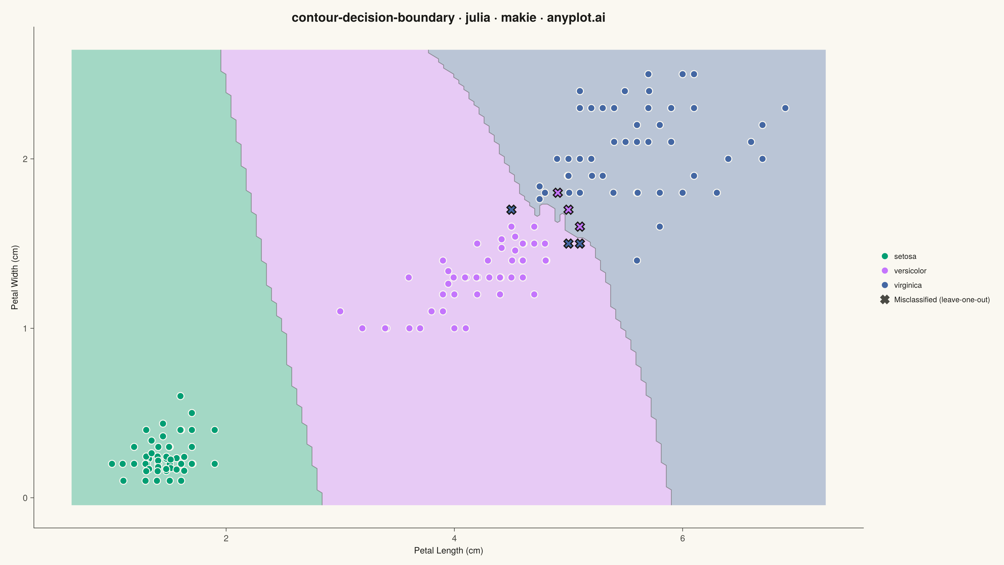
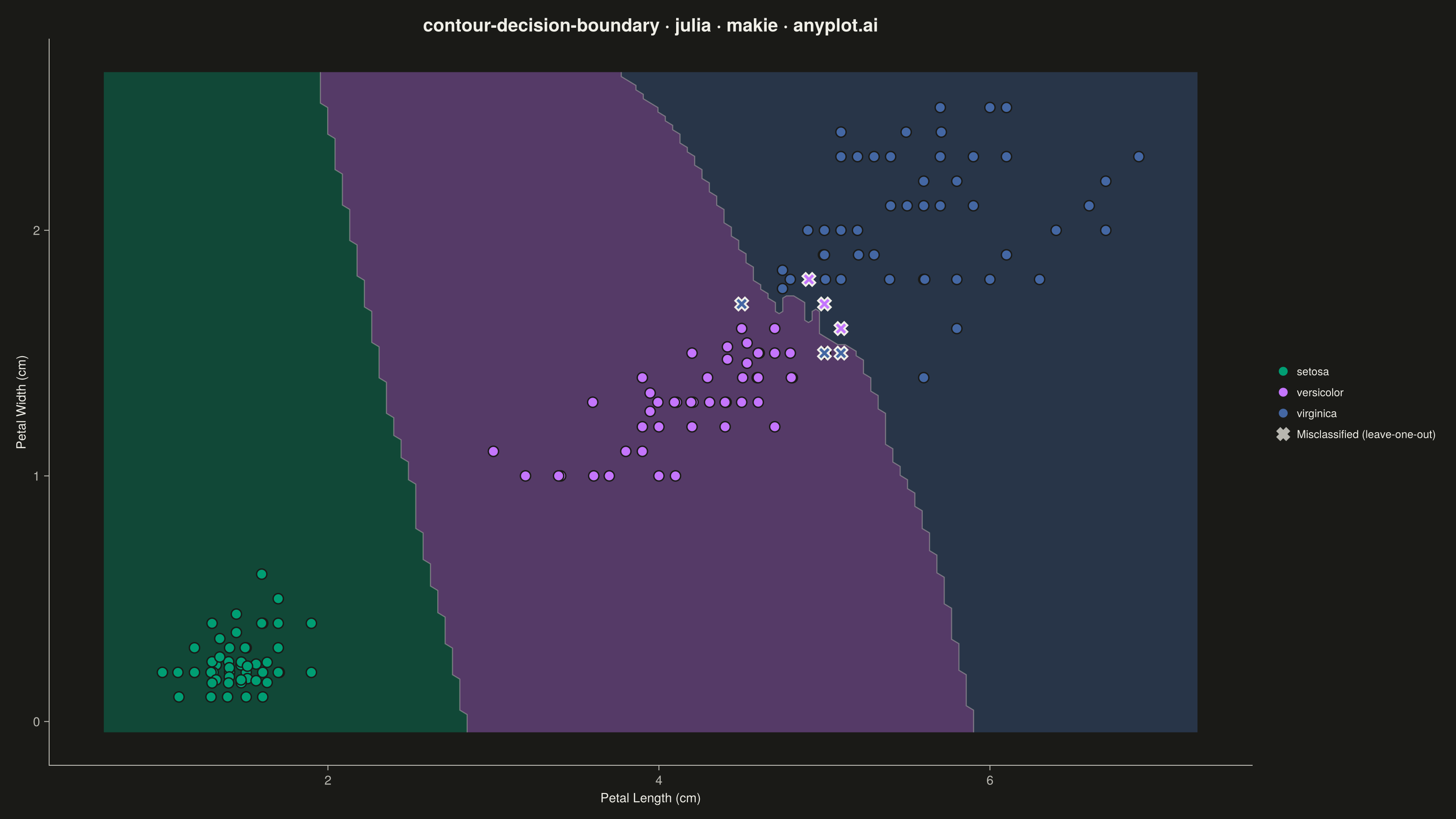
A decision boundary visualization showing how a classifier partitions 2D feature space into predicted class regions. Colored regions indicate the predicted class at each point in the feature space, with training data points overlaid to show how well the classifier separates different classes. This visualization is essential for understanding classifier behavior, identifying decision boundaries, and evaluating classification accuracy in machine learning.
# anyplot.ai
# contour-decision-boundary: Decision Boundary Classifier Visualization
# Library: makie 0.21.9 | Julia 1.11.9
# Quality: 92/100 | Created: 2026-09-04

using CairoMakie
using Colors
using Random
using RDatasets
using DataFrames

Random.seed!(42)

# --- Theme tokens ------------------------------------------------------------
THEME    = get(ENV, "ANYPLOT_THEME", "light")
PAGE_BG  = THEME == "light" ? colorant"#FAF8F1" : colorant"#1A1A17"
INK      = THEME == "light" ? colorant"#1A1A17" : colorant"#F0EFE8"
INK_SOFT = THEME == "light" ? colorant"#4A4A44" : colorant"#B8B7B0"
IMPRINT_PALETTE = [colorant"#009E73", colorant"#C475FD", colorant"#4467A3"]

# --- Data: Fisher's iris, petal measurements for 3 species -------------------
iris = RDatasets.dataset("datasets", "iris")
petal_length = iris.PetalLength
petal_width = iris.PetalWidth
species_labels = String.(iris.Species)
class_names = sort(unique(species_labels))
species_idx = [findfirst(==(s), class_names) for s in species_labels]
n_classes = length(class_names)

# --- Classifier: k-nearest-neighbours vote over a dense mesh grid ------------
k = 9
pad_x = 0.06 * (maximum(petal_length) - minimum(petal_length))
pad_y = 0.06 * (maximum(petal_width) - minimum(petal_width))
xs = range(minimum(petal_length) - pad_x, maximum(petal_length) + pad_x; length = 150)
ys = range(minimum(petal_width) - pad_y, maximum(petal_width) + pad_y; length = 150)

region = Matrix{Int}(undef, length(xs), length(ys))
for (i, gx) in enumerate(xs), (j, gy) in enumerate(ys)
    dist_sq = (petal_length .- gx) .^ 2 .+ (petal_width .- gy) .^ 2
    nearest = partialsortperm(dist_sq, 1:k)
    votes = [count(==(c), species_idx[nearest]) for c in 1:n_classes]
    region[i, j] = argmax(votes)
end

# Leave-one-out re-classification of the training points themselves, to flag
# which ones the classifier gets wrong (used for the marker-shape encoding).
correctly_classified = falses(length(species_idx))
for p in eachindex(species_idx)
    dist_sq = (petal_length .- petal_length[p]) .^ 2 .+ (petal_width .- petal_width[p]) .^ 2
    dist_sq[p] = Inf
    nearest = partialsortperm(dist_sq, 1:k)
    votes = [count(==(c), species_idx[nearest]) for c in 1:n_classes]
    correctly_classified[p] = argmax(votes) == species_idx[p]
end

# Deterministic jitter for exact-duplicate (petal_length, petal_width) pairs so
# that overlapping hit/miss markers don't collapse into a single confusing
# glyph. Classification above uses the true coordinates; only the plotted
# marker positions are nudged.
plot_x = copy(petal_length)
plot_y = copy(petal_width)
duplicate_groups = Dict{Tuple{Float64,Float64},Vector{Int}}()
for (i, key) in enumerate(zip(petal_length, petal_width))
    push!(get!(duplicate_groups, key, Int[]), i)
end
jitter_rx = 0.018 * (maximum(petal_length) - minimum(petal_length))
jitter_ry = 0.018 * (maximum(petal_width) - minimum(petal_width))
for idxs in values(duplicate_groups)
    n_dup = length(idxs)
    if n_dup > 1
        for (rank, i) in enumerate(idxs)
            angle = 2π * (rank - 1) / n_dup
            plot_x[i] += jitter_rx * cos(angle)
            plot_y[i] += jitter_ry * sin(angle)
        end
    end
end

# --- Plot ---------------------------------------------------------------------
fig = Figure(size = (1600, 900), fontsize = 14, backgroundcolor = PAGE_BG)

ax = Axis(
    fig[1, 1];
    title = "contour-decision-boundary · julia · makie · anyplot.ai",
    titlesize = 20,
    titlecolor = INK,
    xlabel = "Petal Length (cm)",
    ylabel = "Petal Width (cm)",
    xlabelsize = 14,
    ylabelsize = 14,
    xlabelcolor = INK,
    ylabelcolor = INK,
    xticklabelsize = 14,
    yticklabelsize = 14,
    xticklabelcolor = INK_SOFT,
    yticklabelcolor = INK_SOFT,
    xtickcolor = INK_SOFT,
    ytickcolor = INK_SOFT,
    backgroundcolor = PAGE_BG,
    topspinevisible = false,
    rightspinevisible = false,
    leftspinecolor = INK_SOFT,
    bottomspinecolor = INK_SOFT,
    xgridvisible = false,
    ygridvisible = false,
)

region_f = Float64.(region)

# Smooth filled decision surface (interpolated boundaries, unlike a blocky
# heatmap!) plus a thin boundary line between adjacent classes for extra
# polish beyond a flat, unrefined region fill.
fill_colors = [RGBAf(c.r, c.g, c.b, 0.35) for c in IMPRINT_PALETTE[1:n_classes]]
contourf!(
    ax, xs, ys, region_f;
    levels = 0.5:1:(n_classes + 0.5),
    colormap = cgrad(fill_colors; categorical = true),
)
contour!(
    ax, xs, ys, region_f;
    levels = collect(1.5:1:(n_classes - 0.5)),
    color = (INK_SOFT, 0.5),
    linewidth = 1.2,
)

for c in 1:n_classes
    in_class = species_idx .== c
    hit = in_class .& correctly_classified
    miss = in_class .& .!correctly_classified
    scatter!(
        ax, plot_x[hit], plot_y[hit];
        color = IMPRINT_PALETTE[c], markersize = 16, marker = :circle,
        strokewidth = 1.5, strokecolor = PAGE_BG, label = class_names[c],
    )
    scatter!(
        ax, plot_x[miss], plot_y[miss];
        color = IMPRINT_PALETTE[c], markersize = 20, marker = :xcross,
        strokewidth = 2, strokecolor = INK,
    )
end

legend_elems = [
    MarkerElement(
        color = IMPRINT_PALETTE[c], marker = :circle, markersize = 16,
        strokewidth = 1.5, strokecolor = PAGE_BG,
    ) for c in 1:n_classes
]
legend_labels = copy(class_names)
push!(legend_elems, MarkerElement(color = INK_SOFT, marker = :xcross, markersize = 18, strokewidth = 2, strokecolor = INK_SOFT))
push!(legend_labels, "Misclassified (leave-one-out)")

Legend(
    fig[1, 2], legend_elems, legend_labels;
    framevisible = false, labelcolor = INK, labelsize = 12,
    backgroundcolor = PAGE_BG,
)

# --- Save ----------------------------------------------------------------------
save("plot-$(THEME).png", fig; px_per_unit = 2)
Runnable source as JSON, for any HTTP client: https://api.anyplot.ai/specs/contour-decision-boundary/makie/code. Any spec id and library id listed in llms-full.txt fit the same URL shape; every URL below is complete and callable.
{
  "spec_id": "contour-decision-boundary",
  "language": "julia",
  "library": "makie",
  "page": "https://anyplot.ai/contour-decision-boundary/julia/makie",
  "hub": "https://anyplot.ai/contour-decision-boundary",
  "code_json": "https://api.anyplot.ai/specs/contour-decision-boundary/makie/code",
  "spec_json": "https://api.anyplot.ai/specs/contour-decision-boundary",
  "render_light_png": "https://storage.googleapis.com/anyplot-images/plots/contour-decision-boundary/julia/makie/plot-light.png",
  "render_dark_png": "https://storage.googleapis.com/anyplot-images/plots/contour-decision-boundary/julia/makie/plot-dark.png",
  "quality_score": 92.0,
  "license": "MIT",
  "guide": "https://anyplot.ai/llms.txt"
}
Part of Decision Boundary Classifier Visualization on anyplot.ai.