The same plot in 14 other libraries — JavaScript: Chart.js, Apache ECharts, Highcharts, MUI X Charts; Python: Altair, Bokeh, lets-plot, Matplotlib, Plotly, plotnine, Pygal, Seaborn; R: ggplot2; Julia: Makie.jl. Compare all 15 side by side: Basic Count Plot in Python, R, Julia and JavaScript.
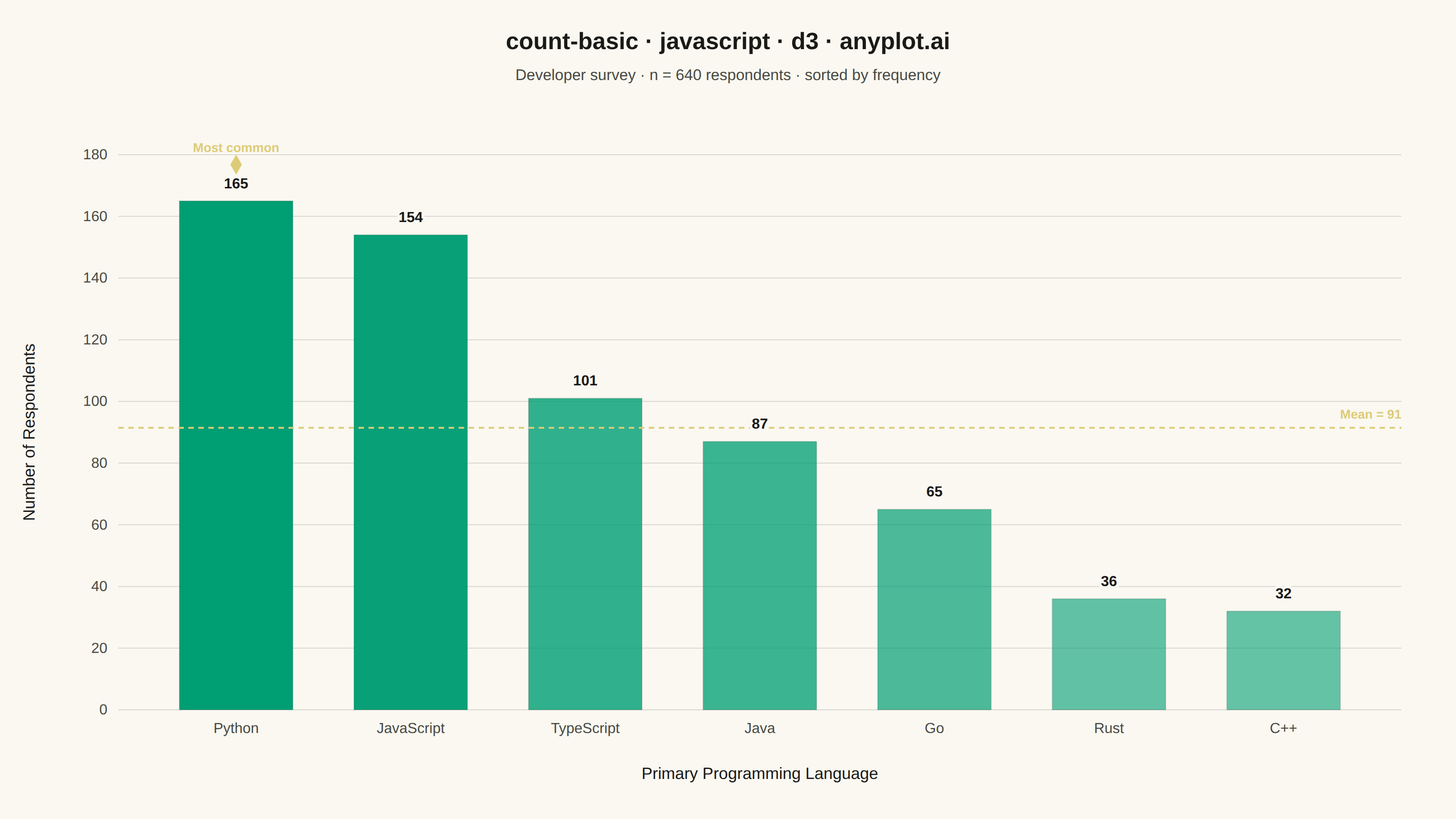
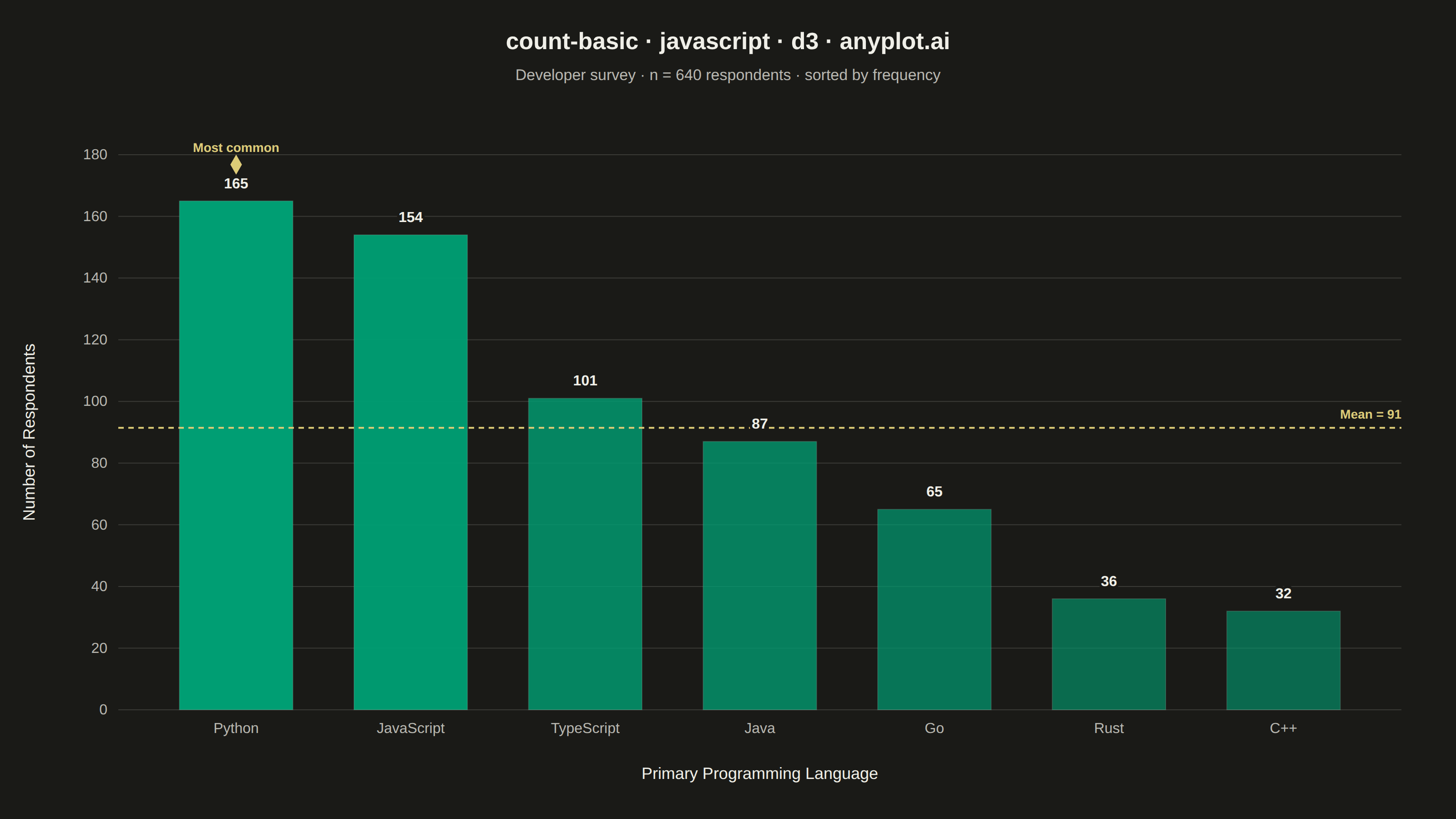
A count plot displays the frequency of observations in each category of a categorical variable using vertical bars. Unlike a basic bar chart that requires pre-computed values, a count plot automatically counts occurrences from raw data. This makes it ideal for quick exploratory analysis of categorical distributions without manual aggregation.
// anyplot.ai
// count-basic: Basic Count Plot
// Library: d3 7.9.0 | JavaScript 22.23.2
// Quality: 88/100 | Updated: 2026-09-30

const t = window.ANYPLOT_TOKENS;
const { width, height } = window.ANYPLOT_SIZE;
const margin = { top: 170, right: 60, bottom: 120, left: 130 };
const iw = width - margin.left - margin.right;
const ih = height - margin.top - margin.bottom;

// --- Data: raw per-respondent observations, counted (not pre-aggregated) ---
// Small LCG so results are deterministic without a browser RNG.
const lcg = (seed) => {
  let state = seed;
  return () => {
    state = (state * 1664525 + 1013904223) % 4294967296;
    return state / 4294967296;
  };
};
const random = lcg(42);

const languageWeights = [
  { language: "Python", weight: 28 },
  { language: "JavaScript", weight: 24 },
  { language: "TypeScript", weight: 16 },
  { language: "Java", weight: 12 },
  { language: "Go", weight: 9 },
  { language: "Rust", weight: 7 },
  { language: "C++", weight: 4 },
];
let cumulative = 0;
const cumulativeWeights = languageWeights.map((d) => {
  cumulative += d.weight;
  return { language: d.language, upTo: cumulative };
});
const totalWeight = cumulative;

const RESPONDENTS = 640;
const surveyResponses = Array.from({ length: RESPONDENTS }, () => {
  const r = random() * totalWeight;
  return cumulativeWeights.find((d) => r <= d.upTo).language;
});

const counts = Array.from(
  d3.rollup(
    surveyResponses,
    (v) => v.length,
    (d) => d,
  ),
  ([language, count]) => ({ language, count }),
).sort((a, b) => d3.descending(a.count, b.count));

// --- SVG mount ---------------------------------------------------------------
const svg = d3.select("#container").append("svg").attr("width", width).attr("height", height);
const g = svg.append("g").attr("transform", `translate(${margin.left},${margin.top})`);

// --- Scales --------------------------------------------------------------------
const x = d3
  .scaleBand()
  .domain(counts.map((d) => d.language))
  .range([0, iw])
  .padding(0.35);
const y = d3
  .scaleLinear()
  .domain([0, d3.max(counts, (d) => d.count)])
  .nice()
  .range([ih, 0]);

// --- Gridlines (y-axis only, subtle) --------------------------------------------
g.append("g")
  .selectAll("line")
  .data(y.ticks(6))
  .join("line")
  .attr("x1", 0)
  .attr("x2", iw)
  .attr("y1", (d) => y(d))
  .attr("y2", (d) => y(d))
  .attr("stroke", t.grid)
  .attr("stroke-width", 1);

// --- Axes ------------------------------------------------------------------------
const xAxis = g
  .append("g")
  .attr("transform", `translate(0,${ih})`)
  .call(d3.axisBottom(x).tickSize(0).tickPadding(14));
const yAxis = g
  .append("g")
  .call(d3.axisLeft(y).ticks(6).tickFormat(d3.format(",d")).tickSize(0).tickPadding(12));
for (const axis of [xAxis, yAxis]) {
  axis.selectAll("text").attr("fill", t.inkSoft).style("font-size", "16px");
  axis.select(".domain").remove();
}
yAxis.selectAll(".tick line").attr("stroke", t.grid);

// --- Bars ---------------------------------------------------------------------
// Single Imprint color at full opacity for every bar, so the data color stays
// identical between themes (no opacity-over-background blending) — the basic
// variant's single categorical variable, per the spec.
g.selectAll("rect")
  .data(counts)
  .join("rect")
  .attr("x", (d) => x(d.language))
  .attr("y", (d) => y(d.count))
  .attr("width", x.bandwidth())
  .attr("height", (d) => ih - y(d.count))
  .attr("fill", t.palette[0])
  .attr("stroke", t.ink)
  .attr("stroke-opacity", 0.15)
  .attr("stroke-width", 1);

// --- Count labels above bars ---------------------------------------------------
g.selectAll(".count-label")
  .data(counts)
  .join("text")
  .attr("class", "count-label")
  .attr("x", (d) => x(d.language) + x.bandwidth() / 2)
  .attr("y", (d) => y(d.count) - 16)
  .attr("text-anchor", "middle")
  .attr("fill", t.ink)
  .style("font-size", "16px")
  .style("font-weight", "600")
  .text((d) => d.count);

// --- Axis titles -----------------------------------------------------------------
g.append("text")
  .attr("x", iw / 2)
  .attr("y", ih + 76)
  .attr("text-anchor", "middle")
  .attr("fill", t.ink)
  .style("font-size", "18px")
  .text("Primary Programming Language");

g.append("text")
  .attr("transform", "rotate(-90)")
  .attr("x", -ih / 2)
  .attr("y", -92)
  .attr("text-anchor", "middle")
  .attr("fill", t.ink)
  .style("font-size", "18px")
  .text("Number of Respondents");

// --- Title -------------------------------------------------------------------
svg
  .append("text")
  .attr("x", width / 2)
  .attr("y", 54)
  .attr("text-anchor", "middle")
  .attr("fill", t.ink)
  .style("font-size", "26px")
  .style("font-weight", "600")
  .text("count-basic · javascript · d3 · anyplot.ai");

svg
  .append("text")
  .attr("x", width / 2)
  .attr("y", 88)
  .attr("text-anchor", "middle")
  .attr("fill", t.inkSoft)
  .style("font-size", "17px")
  .text(`Developer survey · n = ${RESPONDENTS} respondents · sorted by frequency`);
Runnable source as JSON, for any HTTP client: https://api.anyplot.ai/specs/count-basic/d3/code. Any spec id and library id listed in llms-full.txt fit the same URL shape; every URL below is complete and callable.
{
  "spec_id": "count-basic",
  "language": "javascript",
  "library": "d3",
  "page": "https://anyplot.ai/count-basic/javascript/d3",
  "hub": "https://anyplot.ai/count-basic",
  "code_json": "https://api.anyplot.ai/specs/count-basic/d3/code",
  "spec_json": "https://api.anyplot.ai/specs/count-basic",
  "render_light_png": "https://storage.googleapis.com/anyplot-images/plots/count-basic/javascript/d3/plot-light.png",
  "render_dark_png": "https://storage.googleapis.com/anyplot-images/plots/count-basic/javascript/d3/plot-dark.png",
  "interactive_light_html": "https://storage.googleapis.com/anyplot-images/plots/count-basic/javascript/d3/plot-light.html",
  "interactive_dark_html": "https://storage.googleapis.com/anyplot-images/plots/count-basic/javascript/d3/plot-dark.html",
  "quality_score": 88.0,
  "license": "MIT",
  "guide": "https://anyplot.ai/llms.txt"
}
Part of Basic Count Plot on anyplot.ai.