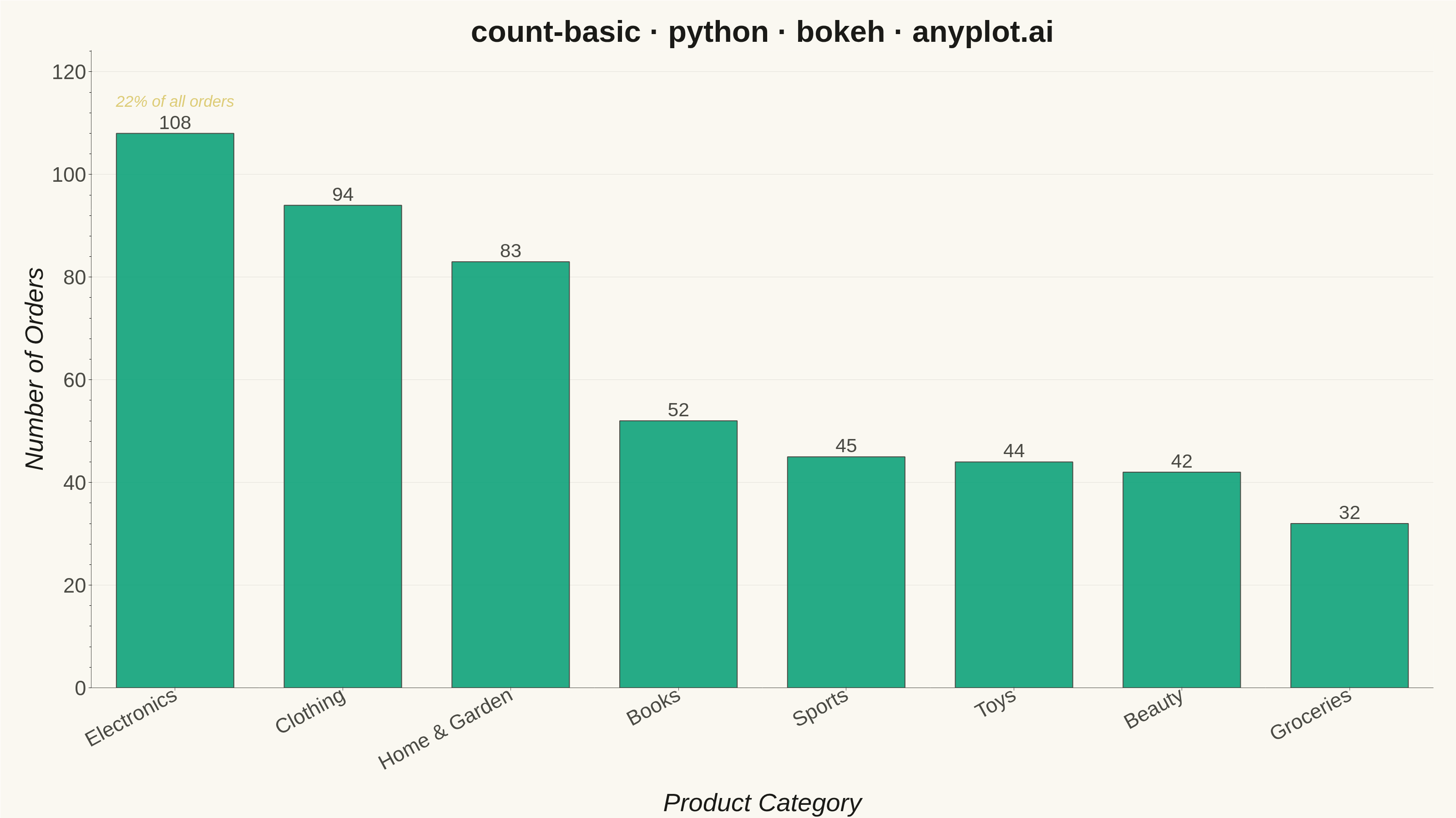
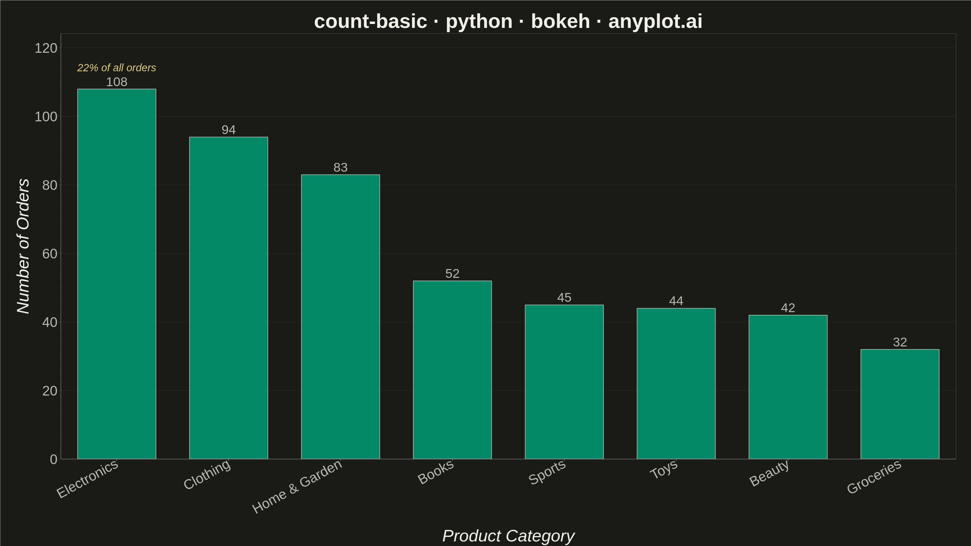
A count plot displays the frequency of observations in each category of a categorical variable using vertical bars. Unlike a basic bar chart that requires pre-computed values, a count plot automatically counts occurrences from raw data. This makes it ideal for quick exploratory analysis of categorical distributions without manual aggregation.
""" anyplot.ai
count-basic: Basic Count Plot
Library: bokeh 3.9.2 | Python 3.13.14
Quality: 91/100 | Updated: 2026-08-11
"""

import os
import sys
import time
from pathlib import Path


sys.path = [p for p in sys.path if "implementations" not in p]

import numpy as np
from bokeh.io import output_file, save
from bokeh.models import ColumnDataSource, HoverTool, LabelSet
from bokeh.plotting import figure
from selenium import webdriver
from selenium.webdriver.chrome.options import Options


# Theme tokens
THEME = os.getenv("ANYPLOT_THEME", "light")
PAGE_BG = "#FAF8F1" if THEME == "light" else "#1A1A17"
ELEVATED_BG = "#FFFDF6" if THEME == "light" else "#242420"
INK = "#1A1A17" if THEME == "light" else "#F0EFE8"
INK_SOFT = "#4A4A44" if THEME == "light" else "#B8B7B0"
BRAND = "#009E73"  # Imprint palette position 1
AMBER = "#DDCC77"  # callout accent, outside the categorical pool

# Data - order counts across product categories in an e-commerce store
np.random.seed(7)
orders = np.random.choice(
    ["Electronics", "Clothing", "Home & Garden", "Books", "Sports", "Toys", "Beauty", "Groceries"],
    size=500,
    p=[0.22, 0.18, 0.15, 0.13, 0.10, 0.08, 0.08, 0.06],
)

# Count occurrences
categories, counts = np.unique(orders, return_counts=True)
# Sort by count descending for better readability
sorted_indices = np.argsort(-counts)
categories = categories[sorted_indices].tolist()
counts = counts[sorted_indices].tolist()
total_orders = sum(counts)
leading_share = counts[0] / total_orders * 100

# Create data source (explicit per-bar fill color list, never a bare scalar,
# so every bar unambiguously resolves to the same brand green)
source = ColumnDataSource(
    data={
        "category": categories,
        "count": counts,
        "label": [str(c) for c in counts],
        "share": [c / total_orders * 100 for c in counts],
        "fill_color": [BRAND] * len(categories),
        "callout": [f"{leading_share:.0f}% of all orders"] + [""] * (len(categories) - 1),
    }
)

# Create figure with categorical x-axis
# `min_border_*` reserve room for the larger 34-42pt chrome so nothing
# clips at the edges of the rendered PNG.
p = figure(
    x_range=categories,
    width=3200,
    height=1800,
    title="count-basic · python · bokeh · anyplot.ai",
    x_axis_label="Product Category",
    y_axis_label="Number of Orders",
    toolbar_location=None,  # avoids the ~30-50px toolbar shrinking the PNG below 3200x1800
    min_border_bottom=160,
    min_border_left=200,
    min_border_top=110,
    min_border_right=50,
)

# Plot bars with brand green — fill_color/line_color set explicitly (not the
# "color=" shorthand) so every bar resolves the same fill unambiguously.
bars = p.vbar(
    x="category",
    top="count",
    source=source,
    width=0.7,
    fill_color="fill_color",
    fill_alpha=0.85,
    line_color=INK_SOFT,
    line_width=2,
    nonselection_fill_color="fill_color",
    nonselection_fill_alpha=0.85,
    nonselection_line_color=INK_SOFT,
)

# Hover detail beyond the bare default — exact count plus each category's
# share of the 500-order sample, without altering the static PNG (the chart
# stays a basic count plot; only the interactive HTML gains this detail).
p.add_tools(
    HoverTool(
        renderers=[bars], tooltips=[("Category", "@category"), ("Orders", "@count"), ("Share of total", "@share{0.0}%")]
    )
)

# Add count labels above bars
labels = LabelSet(
    x="category",
    y="count",
    text="label",
    source=source,
    text_align="center",
    text_baseline="bottom",
    y_offset=10,
    text_font_size="32pt",
    text_color=INK_SOFT,
)
p.add_layout(labels)

# Focal callout on the leading category — surfaces its share of the total
# order volume, adding a storytelling cue beyond plain descending sort.
# Driven off the same categorical source as `labels` (via the "callout"
# column, blank for every row but the leader) rather than a standalone
# `Label`, since bokeh 3.9.2's Label.x rejects a bare categorical factor.
leading_callout = LabelSet(
    x="category",
    y="count",
    text="callout",
    source=source,
    text_align="center",
    text_baseline="bottom",
    y_offset=52,
    text_font_size="26pt",
    text_font_style="italic",
    text_color=AMBER,
)
p.add_layout(leading_callout)

# Style the plot — sizes per prompts/library/bokeh.md "Sizing for 3200x1800"
p.title.text_font_size = "50pt"
p.title.align = "center"
p.title.text_color = INK
p.xaxis.axis_label_text_font_size = "42pt"
p.yaxis.axis_label_text_font_size = "42pt"
p.xaxis.axis_label_text_color = INK
p.yaxis.axis_label_text_color = INK
p.xaxis.major_label_text_font_size = "34pt"
p.yaxis.major_label_text_font_size = "34pt"
p.xaxis.major_label_text_color = INK_SOFT
p.yaxis.major_label_text_color = INK_SOFT

# Grid styling
p.xgrid.grid_line_color = None
p.ygrid.grid_line_color = INK
p.ygrid.grid_line_alpha = 0.10
p.xaxis.axis_line_color = INK_SOFT
p.yaxis.axis_line_color = INK_SOFT
p.xaxis.major_tick_line_color = INK_SOFT
p.yaxis.major_tick_line_color = INK_SOFT

# Axis and background
p.xaxis.major_label_orientation = 0.5
p.y_range.start = 0
p.y_range.end = max(counts) * 1.15
p.background_fill_color = PAGE_BG
p.border_fill_color = PAGE_BG
# No full rectangular outline — rely on the left/bottom axis lines for an
# L-shaped frame, matching the style guide's default spine treatment.
p.outline_line_color = None

# Save files in script directory
script_dir = Path(__file__).parent
html_path = script_dir / f"plot-{THEME}.html"
png_path = script_dir / f"plot-{THEME}.png"

output_file(str(html_path))
save(p)

# Screenshot with headless Chrome
W, H = 3200, 1800
opts = Options()
for arg in (
    "--headless=new",
    "--no-sandbox",
    "--disable-dev-shm-usage",
    "--disable-gpu",
    f"--window-size={W},{H}",
    "--hide-scrollbars",
):
    opts.add_argument(arg)
driver = webdriver.Chrome(options=opts)
driver.set_window_size(W, H)
driver.get(f"file://{html_path.resolve()}")
# Pin the viewport exactly via CDP — headless Chrome's --window-size sets the
# OUTER window, which still reserves a phantom title-bar height even headless.
driver.execute_cdp_cmd(
    "Emulation.setDeviceMetricsOverride", {"width": W, "height": H, "deviceScaleFactor": 1, "mobile": False}
)
time.sleep(3)
driver.save_screenshot(str(png_path))
driver.quit()
Runnable source as JSON, for any HTTP client: https://api.anyplot.ai/specs/count-basic/bokeh/code. Any spec id and library id listed in llms-full.txt fit the same URL shape; every URL below is complete and callable.
{
  "spec_id": "count-basic",
  "language": "python",
  "library": "bokeh",
  "page": "https://anyplot.ai/count-basic/python/bokeh",
  "hub": "https://anyplot.ai/count-basic",
  "code_json": "https://api.anyplot.ai/specs/count-basic/bokeh/code",
  "spec_json": "https://api.anyplot.ai/specs/count-basic",
  "render_light_png": "https://storage.googleapis.com/anyplot-images/plots/count-basic/python/bokeh/plot-light.png",
  "render_dark_png": "https://storage.googleapis.com/anyplot-images/plots/count-basic/python/bokeh/plot-dark.png",
  "interactive_light_html": "https://storage.googleapis.com/anyplot-images/plots/count-basic/python/bokeh/plot-light.html",
  "interactive_dark_html": "https://storage.googleapis.com/anyplot-images/plots/count-basic/python/bokeh/plot-dark.html",
  "quality_score": 91.0,
  "license": "MIT",
  "guide": "https://anyplot.ai/llms.txt"
}
Part of Basic Count Plot on anyplot.ai.