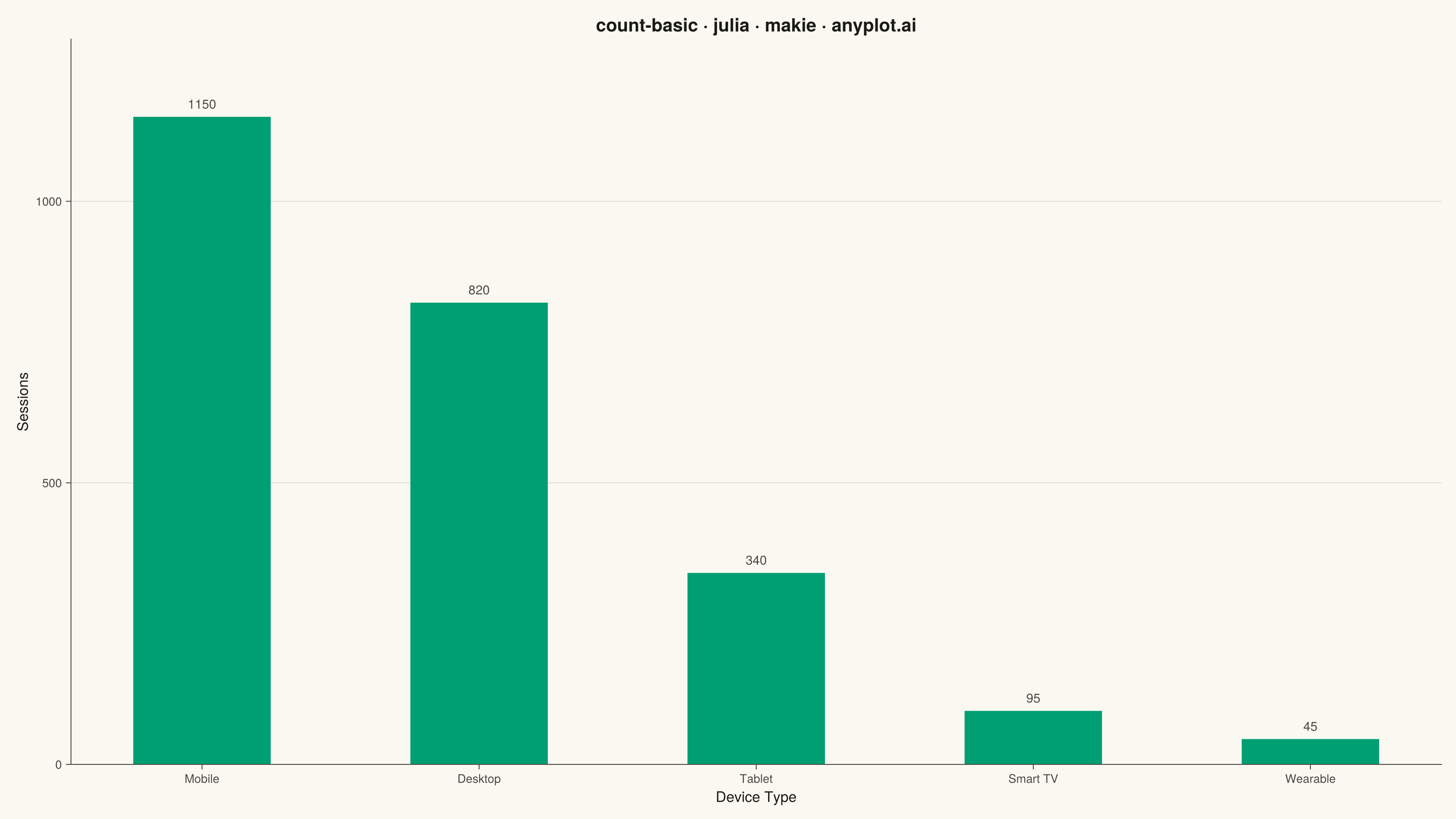
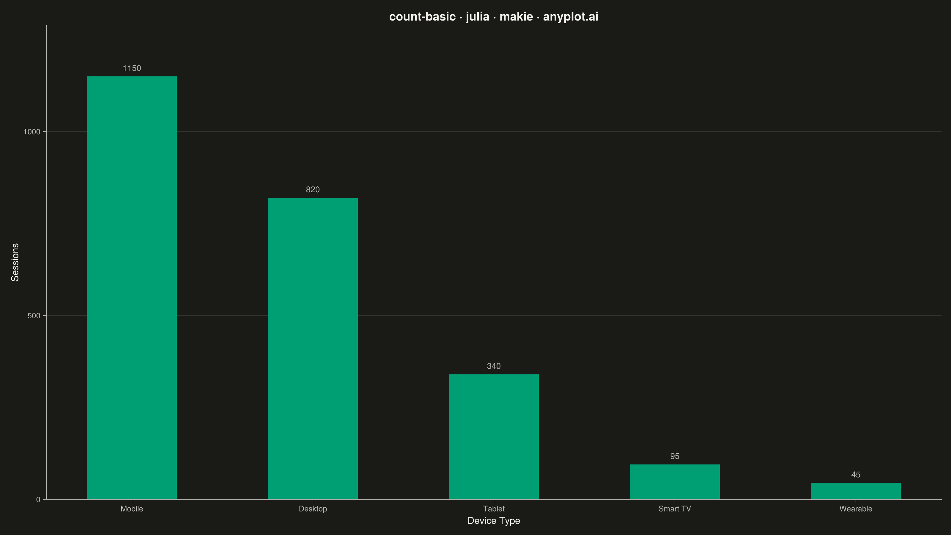
The same plot in 14 other libraries — Python: Altair, Bokeh, lets-plot, Matplotlib, Plotly, plotnine, Pygal, Seaborn; R: ggplot2; JavaScript: Chart.js, D3.js, Apache ECharts, Highcharts, MUI X Charts. Compare all 15 side by side: Basic Count Plot in Python, R, Julia and JavaScript.
A count plot displays the frequency of observations in each category of a categorical variable using vertical bars. Unlike a basic bar chart that requires pre-computed values, a count plot automatically counts occurrences from raw data. This makes it ideal for quick exploratory analysis of categorical distributions without manual aggregation.
# anyplot.ai
# count-basic: Basic Count Plot
# Library: makie 0.21.9 | Julia 1.11.9
# Quality: 82/100 | Updated: 2026-09-27

using CairoMakie
using Colors
using Random

Random.seed!(42)

# --- Theme tokens -----------------------------------------------------------
const THEME    = get(ENV, "ANYPLOT_THEME", "light")
const PAGE_BG  = THEME == "light" ? colorant"#FAF8F1" : colorant"#1A1A17"
const INK      = THEME == "light" ? colorant"#1A1A17" : colorant"#F0EFE8"
const INK_SOFT = THEME == "light" ? colorant"#4A4A44" : colorant"#B8B7B0"
const BRAND    = colorant"#009E73"  # Imprint palette position 1 — ALWAYS first series

# --- Data ---------------------------------------------------------------
# Raw per-session device type from a web analytics log — count-basic tallies
# occurrences from unaggregated observations rather than pre-computed values.
device_types  = ["Desktop", "Mobile", "Tablet", "Smart TV", "Wearable"]
session_share = [820, 1150, 340, 95, 45]  # underlying popularity per device
raw_sessions = reduce(vcat, [fill(device, n) for (device, n) in zip(device_types, session_share)])
shuffle!(raw_sessions)

session_counts = Dict{String,Int}()
for device in raw_sessions
    session_counts[device] = get(session_counts, device, 0) + 1
end

# Sorted by frequency, descending
sorted_devices = sort(collect(keys(session_counts)); by = d -> session_counts[d], rev = true)
sorted_counts  = [session_counts[d] for d in sorted_devices]

# --- Plot -----------------------------------------------------------------
fig = Figure(
    resolution      = (1600, 900),
    fontsize        = 14,
    backgroundcolor = PAGE_BG,
)

ax = Axis(
    fig[1, 1];
    title             = "Device Type Sessions · count-basic · julia · makie · anyplot.ai",
    titlesize         = 20,
    titlecolor        = INK,
    xlabel            = "Device Type",
    ylabel            = "Sessions",
    xlabelsize        = 16,
    ylabelsize        = 16,
    xlabelcolor       = INK,
    ylabelcolor       = INK,
    xticklabelsize    = 13,
    yticklabelsize    = 13,
    xticklabelcolor   = INK_SOFT,
    yticklabelcolor   = INK_SOFT,
    xtickcolor        = INK_SOFT,
    ytickcolor        = INK_SOFT,
    backgroundcolor   = PAGE_BG,
    leftspinecolor    = INK_SOFT,
    bottomspinecolor  = INK_SOFT,
    xgridvisible      = false,
    ygridcolor        = RGBAf(INK.r, INK.g, INK.b, 0.12),
    xticks            = (1:length(sorted_devices), sorted_devices),
)
hidespines!(ax, :t, :r)

barplot!(
    ax, 1:length(sorted_devices), sorted_counts;
    color = BRAND, width = 0.62,
    strokewidth = 1.5, strokecolor = PAGE_BG,
)

total_sessions = sum(sorted_counts)
for (i, count) in enumerate(sorted_counts)
    text!(
        ax, i, count;
        text = string(count),
        align = (:center, :bottom),
        offset = (0, 6),
        fontsize = 14,
        color = INK,
    )
    pct = round(100 * count / total_sessions; digits = 1)
    text!(
        ax, i, count;
        text = "($(pct)%)",
        align = (:center, :bottom),
        offset = (0, 24),
        fontsize = 11,
        color = INK_SOFT,
    )
end

ylims!(ax, 0, maximum(sorted_counts) * 1.2)

# --- Save -------------------------------------------------------------------
save("plot-$(THEME).png", fig; px_per_unit = 2)
Runnable source as JSON, for any HTTP client: https://api.anyplot.ai/specs/count-basic/makie/code. Any spec id and library id listed in llms-full.txt fit the same URL shape; every URL below is complete and callable.
{
  "spec_id": "count-basic",
  "language": "julia",
  "library": "makie",
  "page": "https://anyplot.ai/count-basic/julia/makie",
  "hub": "https://anyplot.ai/count-basic",
  "code_json": "https://api.anyplot.ai/specs/count-basic/makie/code",
  "spec_json": "https://api.anyplot.ai/specs/count-basic",
  "render_light_png": "https://storage.googleapis.com/anyplot-images/plots/count-basic/julia/makie/plot-light.png",
  "render_dark_png": "https://storage.googleapis.com/anyplot-images/plots/count-basic/julia/makie/plot-dark.png",
  "quality_score": 82.0,
  "license": "MIT",
  "guide": "https://anyplot.ai/llms.txt"
}
Part of Basic Count Plot on anyplot.ai.