The same plot in 14 other libraries — JavaScript: Chart.js, Apache ECharts, Highcharts, MUI X Charts; Python: Altair, Bokeh, lets-plot, Matplotlib, Plotly, plotnine, Pygal, Seaborn; R: ggplot2; Julia: Makie.jl. Compare all 15 side by side: Returns Distribution Histogram in Python, R, Julia and JavaScript.
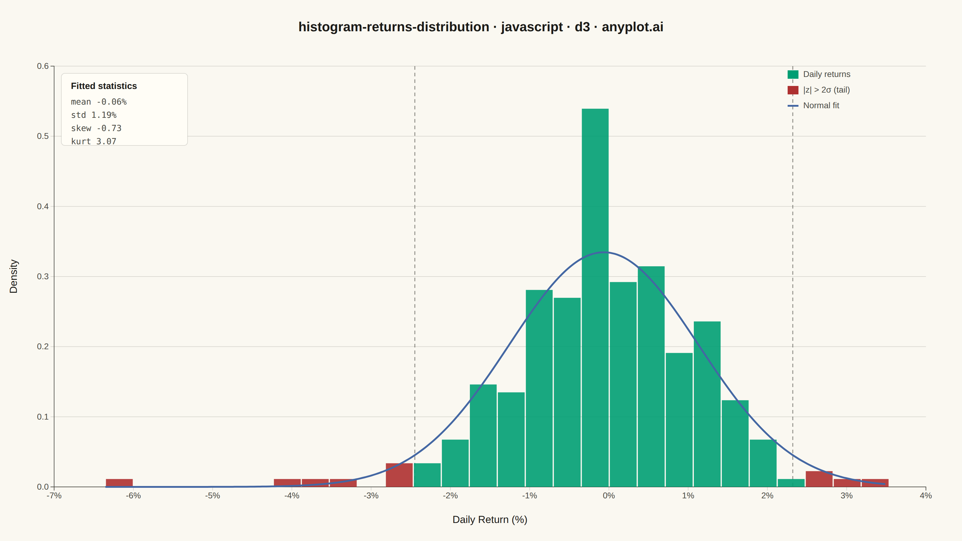
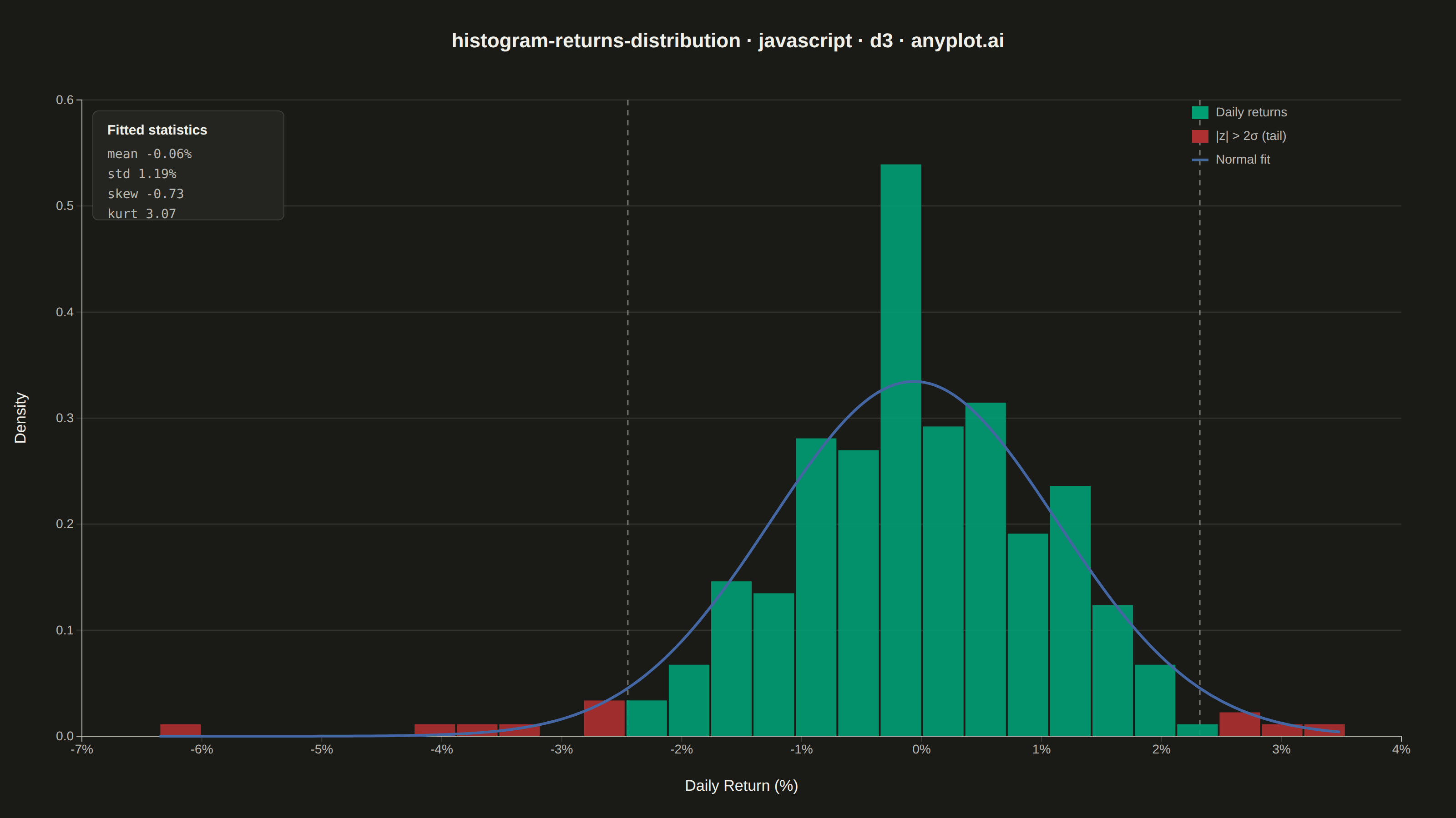
A histogram showing the distribution of financial returns (daily, weekly, or monthly) with a normal distribution overlay for comparison. This visualization is essential for risk analysis, allowing analysts to assess whether returns follow a normal distribution, identify fat tails indicating higher-than-expected extreme events, and measure asymmetry through skewness. Key statistics are displayed directly on the plot for quick interpretation.
// anyplot.ai
// histogram-returns-distribution: Returns Distribution Histogram
// Library: d3 7.9.0 | JavaScript 22.23.2
// Quality: 87/100 | Created: 2026-09-02

const t = window.ANYPLOT_TOKENS;
const { width, height } = window.ANYPLOT_SIZE;
const margin = { top: 110, right: 60, bottom: 90, left: 90 };
const iw = width - margin.left - margin.right;
const ih = height - margin.top - margin.bottom;

// --- Data: 252 daily returns (%) from a fixed-seed mixture -----------------
// 92% "calm" days ~ N(0.05, 1.05); 8% "shock" days ~ N(-2.1, 2.6) — the
// mixture produces the negative skew and fat left tail typical of equity
// return series without relying on an unseeded RNG.
let lcgState = 20260902;
function uniform() {
  lcgState = (1103515245 * lcgState + 12345) % 2147483648;
  return lcgState / 2147483648;
}
function gaussian() {
  const u1 = Math.max(uniform(), 1e-9);
  const u2 = uniform();
  return Math.sqrt(-2 * Math.log(u1)) * Math.cos(2 * Math.PI * u2);
}

const n = 252;
const returns = [];
for (let i = 0; i < n; i++) {
  const shock = uniform() < 0.08;
  const value = shock ? -2.1 + gaussian() * 2.6 : 0.05 + gaussian() * 1.05;
  returns.push(value);
}

// --- Fitted statistics --------------------------------------------------
const meanVal = d3.mean(returns);
const stdVal = d3.deviation(returns);
const skew =
  d3.sum(returns, (d) => Math.pow((d - meanVal) / stdVal, 3)) / n;
const kurt =
  d3.sum(returns, (d) => Math.pow((d - meanVal) / stdVal, 4)) / n - 3;

// --- Histogram (density-normalized, equal-width bins) -----------------------
// Binned manually (rather than d3.bin()'s default "nice" thresholds) so every
// bin has the exact same width — d3.bin()'s rounded edge thresholds can leave
// the first/last bin narrower than the rest, which would distort a lone
// tail observation into a misleadingly tall density spike.
const [dataMin, dataMax] = d3.extent(returns);
const numBins = 28;
const binWidth = (dataMax - dataMin) / numBins;
const density = d3.range(numBins).map((i) => {
  const x0 = dataMin + i * binWidth;
  const x1 = x0 + binWidth;
  const count = returns.filter((v) => v >= x0 && (v < x1 || (i === numBins - 1 && v <= x1))).length;
  return { x0, x1, y: count / (n * binWidth) };
});

// --- Normal curve fitted to mean/std ----------------------------------------
function normalPdf(x) {
  return (
    Math.exp(-0.5 * Math.pow((x - meanVal) / stdVal, 2)) /
    (stdVal * Math.sqrt(2 * Math.PI))
  );
}
const curveX = d3.range(dataMin, dataMax, (dataMax - dataMin) / 200);
const curvePoints = curveX.map((x) => ({ x, y: normalPdf(x) }));

// --- Scales -------------------------------------------------------------
const x = d3.scaleLinear().domain([dataMin, dataMax]).nice().range([0, iw]);
const yMax = Math.max(d3.max(density, (d) => d.y), d3.max(curvePoints, (d) => d.y)) * 1.1;
const y = d3.scaleLinear().domain([0, yMax]).nice().range([ih, 0]);

// --- SVG mount ------------------------------------------------------------
const svg = d3.select("#container").append("svg").attr("width", width).attr("height", height);
const g = svg.append("g").attr("transform", `translate(${margin.left},${margin.top})`);

// --- Axes -----------------------------------------------------------------
const xAxis = g
  .append("g")
  .attr("transform", `translate(0,${ih})`)
  .call(d3.axisBottom(x).tickFormat((d) => `${d}%`).ticks(10));
const yAxis = g.append("g").call(d3.axisLeft(y).ticks(6));
for (const ax of [xAxis, yAxis]) {
  ax.selectAll("text").attr("fill", t.inkSoft).style("font-size", "14px");
  ax.selectAll("line").attr("stroke", t.grid);
  ax.select(".domain").attr("stroke", t.inkSoft);
}

// y-axis gridlines (subtle, matches "both axes for continuous/scatter-like" density plot)
g.append("g")
  .attr("class", "grid")
  .call(d3.axisLeft(y).ticks(6).tickSize(-iw).tickFormat(""))
  .selectAll("line")
  .attr("stroke", t.grid);
g.select(".grid .domain").remove();

// --- Tail boundary reference lines (±2σ) ------------------------------------
const tailLo = meanVal - 2 * stdVal;
const tailHi = meanVal + 2 * stdVal;
for (const bound of [tailLo, tailHi]) {
  g.append("line")
    .attr("x1", x(bound)).attr("x2", x(bound))
    .attr("y1", 0).attr("y2", ih)
    .attr("stroke", t.inkSoft)
    .attr("stroke-width", 1.5)
    .attr("stroke-dasharray", "6,5")
    .attr("opacity", 0.6);
}

// --- Histogram bars: green for the bulk, matte red beyond ±2σ --------------
g.selectAll("rect.bar")
  .data(density)
  .join("rect")
  .attr("class", "bar")
  .attr("x", (d) => x(d.x0) + 1)
  .attr("y", (d) => y(d.y))
  .attr("width", (d) => Math.max(x(d.x1) - x(d.x0) - 2, 0))
  .attr("height", (d) => ih - y(d.y))
  .attr("fill", (d) => {
    const center = (d.x0 + d.x1) / 2;
    return center < tailLo || center > tailHi ? t.palette[4] : t.palette[0];
  })
  .attr("opacity", 0.9);

// --- Fitted normal curve ----------------------------------------------------
const line = d3.line().x((d) => x(d.x)).y((d) => y(d.y)).curve(d3.curveBasis);
g.append("path")
  .datum(curvePoints)
  .attr("fill", "none")
  .attr("stroke", t.palette[2])
  .attr("stroke-width", 3)
  .attr("d", line);

// --- Axis titles --------------------------------------------------------
g.append("text")
  .attr("x", iw / 2).attr("y", ih + 60)
  .attr("text-anchor", "middle")
  .attr("fill", t.ink).style("font-size", "17px")
  .text("Daily Return (%)");
g.append("text")
  .attr("transform", "rotate(-90)")
  .attr("x", -ih / 2).attr("y", -62)
  .attr("text-anchor", "middle")
  .attr("fill", t.ink).style("font-size", "17px")
  .text("Density");

// --- Legend -----------------------------------------------------------------
const legend = [
  { label: "Daily returns", swatch: t.palette[0] },
  { label: "|z| > 2σ (tail)", swatch: t.palette[4] },
  { label: "Normal fit", swatch: t.palette[2], line: true },
];
const legendG = g.append("g").attr("transform", `translate(${iw - 230}, 6)`);
legend.forEach((item, i) => {
  const row = legendG.append("g").attr("transform", `translate(0, ${i * 26})`);
  if (item.line) {
    row.append("line").attr("x1", 0).attr("x2", 18).attr("y1", 8).attr("y2", 8)
      .attr("stroke", item.swatch).attr("stroke-width", 3);
  } else {
    row.append("rect").attr("width", 18).attr("height", 14).attr("y", 1).attr("fill", item.swatch);
  }
  row.append("text").attr("x", 26).attr("y", 12)
    .attr("fill", t.inkSoft).style("font-size", "14px")
    .text(item.label);
});

// --- Statistics callout box --------------------------------------------------
const statLines = [
  `mean  ${meanVal >= 0 ? "+" : ""}${meanVal.toFixed(2)}%`,
  `std       ${stdVal.toFixed(2)}%`,
  `skew    ${skew.toFixed(2)}`,
  `kurt     ${kurt.toFixed(2)}`,
];
const boxW = 210;
const boxH = 24 * statLines.length + 24;
const boxG = g.append("g").attr("transform", `translate(12, 12)`);
boxG.append("rect")
  .attr("width", boxW).attr("height", boxH)
  .attr("fill", t.elevatedBg)
  .attr("stroke", t.grid)
  .attr("rx", 6);
boxG.append("text")
  .attr("x", 16).attr("y", 26)
  .attr("fill", t.ink).style("font-size", "15px").style("font-weight", "600")
  .text("Fitted statistics");
statLines.forEach((line, i) => {
  boxG.append("text")
    .attr("x", 16).attr("y", 52 + i * 22)
    .attr("fill", t.inkSoft).style("font-size", "14px")
    .style("font-family", "monospace")
    .text(line);
});

// --- Title ------------------------------------------------------------------
svg.append("text")
  .attr("x", width / 2).attr("y", 52)
  .attr("text-anchor", "middle")
  .attr("fill", t.ink).style("font-size", "22px").style("font-weight", "600")
  .text("histogram-returns-distribution · javascript · d3 · anyplot.ai");
Runnable source as JSON, for any HTTP client: https://api.anyplot.ai/specs/histogram-returns-distribution/d3/code. Any spec id and library id listed in llms-full.txt fit the same URL shape; every URL below is complete and callable.
{
  "spec_id": "histogram-returns-distribution",
  "language": "javascript",
  "library": "d3",
  "page": "https://anyplot.ai/histogram-returns-distribution/javascript/d3",
  "hub": "https://anyplot.ai/histogram-returns-distribution",
  "code_json": "https://api.anyplot.ai/specs/histogram-returns-distribution/d3/code",
  "spec_json": "https://api.anyplot.ai/specs/histogram-returns-distribution",
  "render_light_png": "https://storage.googleapis.com/anyplot-images/plots/histogram-returns-distribution/javascript/d3/plot-light.png",
  "render_dark_png": "https://storage.googleapis.com/anyplot-images/plots/histogram-returns-distribution/javascript/d3/plot-dark.png",
  "interactive_light_html": "https://storage.googleapis.com/anyplot-images/plots/histogram-returns-distribution/javascript/d3/plot-light.html",
  "interactive_dark_html": "https://storage.googleapis.com/anyplot-images/plots/histogram-returns-distribution/javascript/d3/plot-dark.html",
  "quality_score": 87.0,
  "license": "MIT",
  "guide": "https://anyplot.ai/llms.txt"
}
Part of Returns Distribution Histogram on anyplot.ai.