The same plot in 14 other libraries — Python: Altair, Bokeh, lets-plot, Matplotlib, Plotly, plotnine, Pygal, Seaborn; R: ggplot2; JavaScript: Chart.js, D3.js, Apache ECharts, Highcharts, MUI X Charts. Compare all 15 side by side: Returns Distribution Histogram in Python, R, Julia and JavaScript.
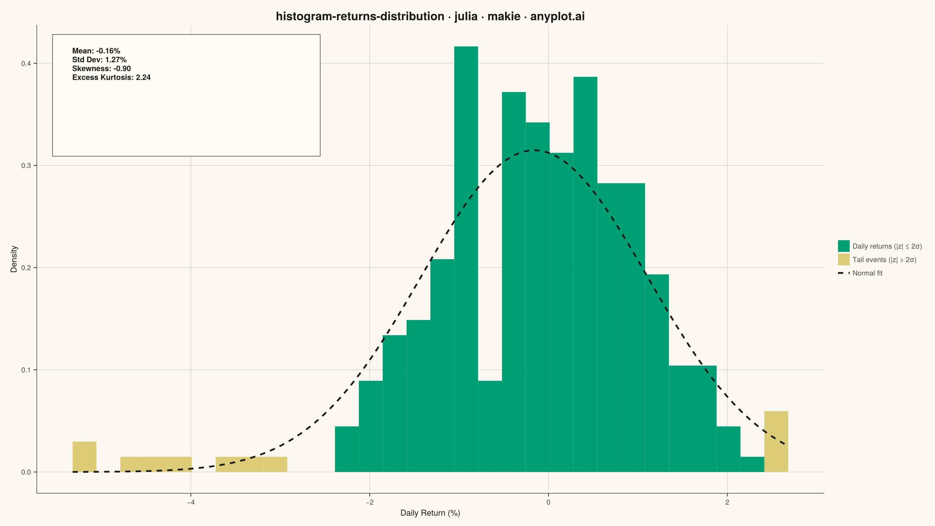
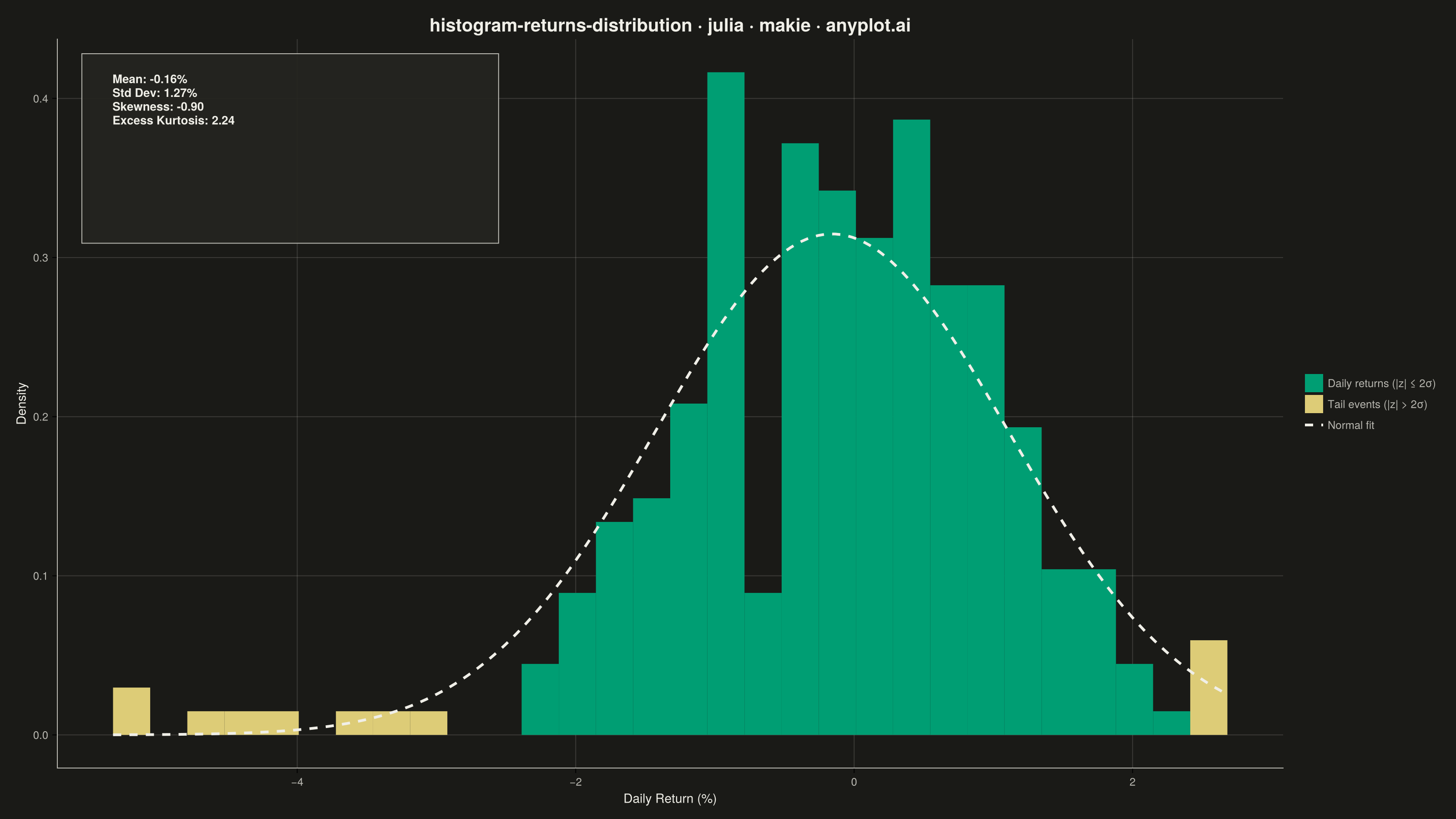
A histogram showing the distribution of financial returns (daily, weekly, or monthly) with a normal distribution overlay for comparison. This visualization is essential for risk analysis, allowing analysts to assess whether returns follow a normal distribution, identify fat tails indicating higher-than-expected extreme events, and measure asymmetry through skewness. Key statistics are displayed directly on the plot for quick interpretation.
# anyplot.ai
# histogram-returns-distribution: Returns Distribution Histogram
# Library: makie 0.21.9 | Julia 1.11.9
# Quality: 92/100 | Created: 2026-09-02

using CairoMakie
using Colors
using Random
using Statistics
using Printf

Random.seed!(42)

# --- Theme tokens -------------------------------------------------------------
const THEME       = get(ENV, "ANYPLOT_THEME", "light")
const PAGE_BG     = THEME == "light" ? colorant"#FAF8F1" : colorant"#1A1A17"
const ELEVATED_BG = THEME == "light" ? colorant"#FFFDF6" : colorant"#242420"
const INK         = THEME == "light" ? colorant"#1A1A17" : colorant"#F0EFE8"
const INK_SOFT    = THEME == "light" ? colorant"#4A4A44" : colorant"#B8B7B0"
const IMPRINT_PALETTE = [
    colorant"#009E73", colorant"#C475FD", colorant"#4467A3", colorant"#BD8233",
    colorant"#AE3030", colorant"#2ABCCD", colorant"#954477", colorant"#99B314",
]
const ANYPLOT_AMBER = colorant"#DDCC77"  # warning — tail events beyond 2 std dev
const ANYPLOT_NEUTRAL = INK             # reference line — fitted normal curve

# --- Data -----------------------------------------------------------------
# One trading year of daily ETF returns (%). A minority of days carry a larger
# negative shock, producing the fat left tail and mild negative skew typical
# of real equity return series.
n_days = 252
base_returns = 1.1 .* randn(n_days) .+ 0.05
is_shock_day = rand(n_days) .< 0.07
crash_shocks = -abs.(2.6 .* randn(n_days))
daily_returns = ifelse.(is_shock_day, base_returns .+ crash_shocks, base_returns)

mean_return = mean(daily_returns)
std_return = std(daily_returns)
z_scores = (daily_returns .- mean_return) ./ std_return
skewness = mean(z_scores .^ 3)
excess_kurtosis = mean(z_scores .^ 4) - 3

# --- Histogram binning (manual, so tail bins can be recolored) ------------
n_bins = 22
lo, hi = minimum(daily_returns), maximum(daily_returns)
edges = range(lo, hi; length = n_bins + 1)
bin_width = step(edges)
counts = zeros(Int, n_bins)
for r in daily_returns
    idx = clamp(Int(floor((r - lo) / bin_width)) + 1, 1, n_bins)
    counts[idx] += 1
end
bin_centers = [edges[i] + bin_width / 2 for i in 1:n_bins]
densities = counts ./ (n_days * bin_width)  # density normalization

tail_threshold = 2 * std_return
is_tail_bin = [abs(c - mean_return) > tail_threshold for c in bin_centers]

# Normal distribution fitted to the sample, for comparison
normal_xs = range(lo, hi; length = 200)
normal_pdf(x) = exp(-0.5 * ((x - mean_return) / std_return)^2) / (std_return * sqrt(2π))
normal_ys = normal_pdf.(normal_xs)

# --- Plot -------------------------------------------------------------------
fig = Figure(
    resolution      = (1600, 900),
    fontsize        = 14,
    backgroundcolor = PAGE_BG,
)

ax = Axis(
    fig[1, 1];
    title              = "histogram-returns-distribution · julia · makie · anyplot.ai",
    titlesize          = 25,
    titlecolor         = INK,
    xlabel             = "Daily Return (%)",
    ylabel             = "Density",
    xlabelsize         = 14,
    ylabelsize         = 14,
    xlabelcolor        = INK,
    ylabelcolor        = INK,
    xticklabelsize     = 12,
    yticklabelsize     = 12,
    xticklabelcolor    = INK_SOFT,
    yticklabelcolor    = INK_SOFT,
    backgroundcolor    = PAGE_BG,
    topspinevisible    = false,
    rightspinevisible  = false,
    leftspinecolor     = INK_SOFT,
    bottomspinecolor   = INK_SOFT,
    xgridcolor         = RGBAf(INK.r, INK.g, INK.b, 0.15),
    ygridcolor         = RGBAf(INK.r, INK.g, INK.b, 0.15),
    xminorgridvisible  = false,
    yminorgridvisible  = false,
)

barplot!(
    ax, bin_centers[.!is_tail_bin], densities[.!is_tail_bin];
    color = IMPRINT_PALETTE[1], width = bin_width, gap = 0.0,
    label = "Daily returns (|z| ≤ 2σ)",
)
barplot!(
    ax, bin_centers[is_tail_bin], densities[is_tail_bin];
    color = ANYPLOT_AMBER, width = bin_width, gap = 0.0,
    label = "Tail events (|z| > 2σ)",
)
lines!(
    ax, normal_xs, normal_ys;
    color = ANYPLOT_NEUTRAL, linewidth = 3, linestyle = :dash, label = "Normal fit",
)

# Legend built declaratively from the axis's own labeled plot objects, rather
# than hand-assembled proxy elements — Makie collects the legend entries for us.
Legend(
    fig[1, 2], ax;
    framevisible = false,
    labelcolor   = INK_SOFT,
    labelsize    = 12,
    backgroundcolor = PAGE_BG,
)

stats_text = @sprintf(
    "Mean: %.2f%%\nStd Dev: %.2f%%\nSkewness: %.2f\nExcess Kurtosis: %.2f",
    mean_return, std_return, skewness, excess_kurtosis,
)
poly!(
    ax, Rect2f(0.02, 0.79, 0.34, 0.17);
    color = (ELEVATED_BG, 0.92), strokecolor = INK_SOFT, strokewidth = 1,
    space = :relative,
)
text!(
    ax, 0.045, 0.935;
    text = stats_text, space = :relative, align = (:left, :top),
    color = INK, fontsize = 13, font = :bold,
)

# --- Save -------------------------------------------------------------------
save("plot-$(THEME).png", fig; px_per_unit = 2)
Runnable source as JSON, for any HTTP client: https://api.anyplot.ai/specs/histogram-returns-distribution/makie/code. Any spec id and library id listed in llms-full.txt fit the same URL shape; every URL below is complete and callable.
{
  "spec_id": "histogram-returns-distribution",
  "language": "julia",
  "library": "makie",
  "page": "https://anyplot.ai/histogram-returns-distribution/julia/makie",
  "hub": "https://anyplot.ai/histogram-returns-distribution",
  "code_json": "https://api.anyplot.ai/specs/histogram-returns-distribution/makie/code",
  "spec_json": "https://api.anyplot.ai/specs/histogram-returns-distribution",
  "render_light_png": "https://storage.googleapis.com/anyplot-images/plots/histogram-returns-distribution/julia/makie/plot-light.png",
  "render_dark_png": "https://storage.googleapis.com/anyplot-images/plots/histogram-returns-distribution/julia/makie/plot-dark.png",
  "quality_score": 92.0,
  "license": "MIT",
  "guide": "https://anyplot.ai/llms.txt"
}
Part of Returns Distribution Histogram on anyplot.ai.