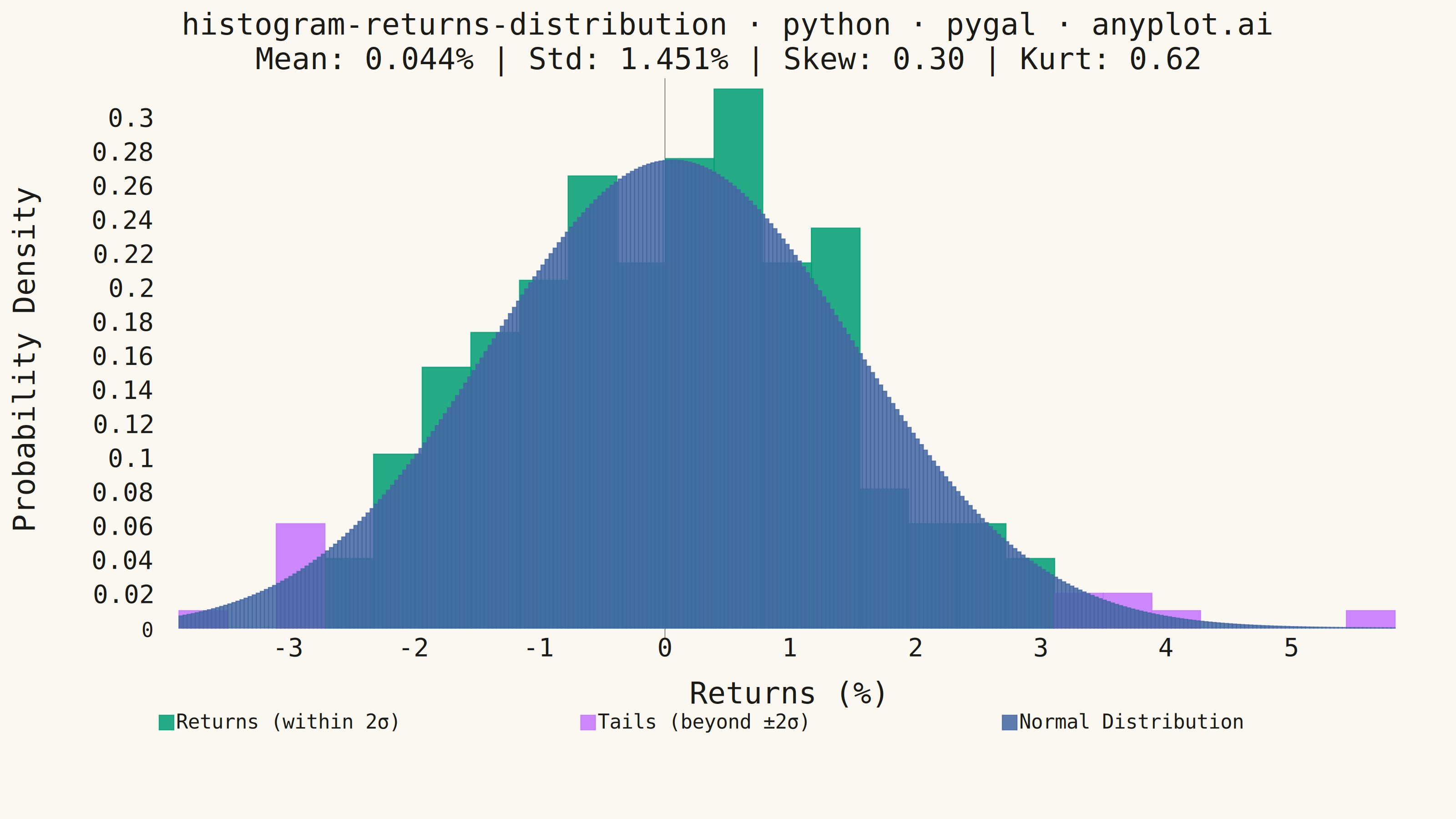
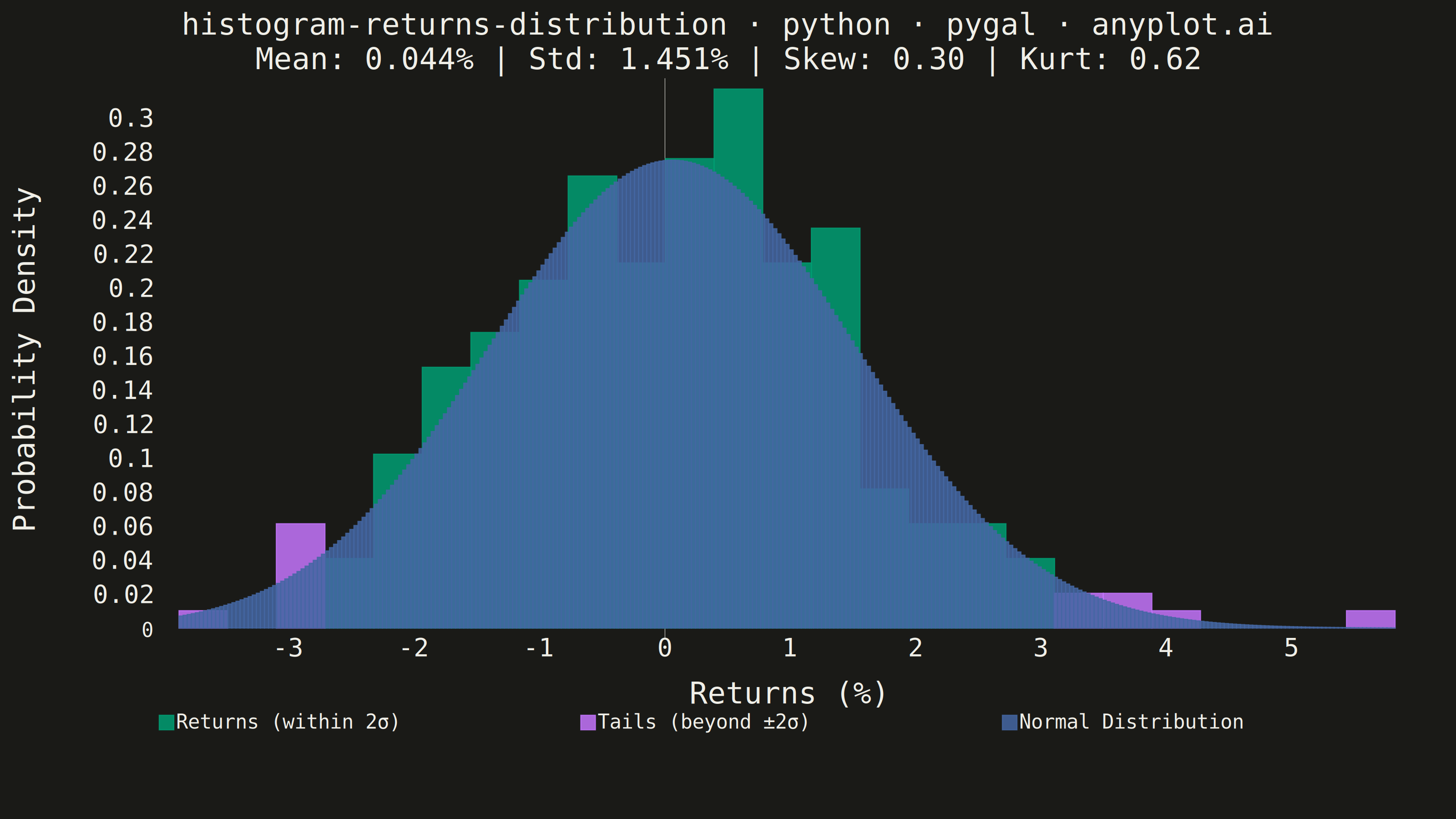
A histogram showing the distribution of financial returns (daily, weekly, or monthly) with a normal distribution overlay for comparison. This visualization is essential for risk analysis, allowing analysts to assess whether returns follow a normal distribution, identify fat tails indicating higher-than-expected extreme events, and measure asymmetry through skewness. Key statistics are displayed directly on the plot for quick interpretation.
""" anyplot.ai
histogram-returns-distribution: Returns Distribution Histogram
Library: pygal 3.1.0 | Python 3.13.13
Quality: 88/100 | Updated: 2026-05-20
"""

import sys


sys.path.pop(0)  # Prevent self-import: pygal.py shadows the installed pygal package

import os

import numpy as np
import pygal
from pygal.style import Style


THEME = os.getenv("ANYPLOT_THEME", "light")
PAGE_BG = "#FAF8F1" if THEME == "light" else "#1A1A17"
INK = "#1A1A17" if THEME == "light" else "#F0EFE8"
INK_MUTED = "#6B6A63" if THEME == "light" else "#A8A79F"

IMPRINT = ("#009E73", "#C475FD", "#4467A3", "#BD8233", "#AE3030", "#2ABCCD", "#954477")

# Data — 252 daily stock returns (1 trading year)
np.random.seed(42)
returns = np.random.normal(loc=0.0005, scale=0.015, size=252) * 100  # as percentage

n = len(returns)
mean_return = np.mean(returns)
std_return = np.std(returns, ddof=1)
skewness = (n / ((n - 1) * (n - 2))) * np.sum(((returns - mean_return) / std_return) ** 3)
kurtosis = ((n * (n + 1)) / ((n - 1) * (n - 2) * (n - 3))) * np.sum(((returns - mean_return) / std_return) ** 4) - (
    3 * (n - 1) ** 2
) / ((n - 2) * (n - 3))

n_bins = 25
counts, bin_edges = np.histogram(returns, bins=n_bins, density=True)

lower_tail = mean_return - 2 * std_return
upper_tail = mean_return + 2 * std_return

# Histogram bars: pygal.Histogram native format (value, xmin, xmax)
normal_bars = []
tail_bars = []
for i, count in enumerate(counts):
    left = float(bin_edges[i])
    right = float(bin_edges[i + 1])
    center = (left + right) / 2
    height = float(count)
    bar = (height, left, right)
    if center < lower_tail or center > upper_tail:
        tail_bars.append(bar)
    else:
        normal_bars.append(bar)

# Normal distribution curve — 300 dense adjacent thin bins approximate a smooth overlay
x_curve = np.linspace(float(bin_edges[0]), float(bin_edges[-1]), 300)
normal_pdf = (1 / (std_return * np.sqrt(2 * np.pi))) * np.exp(-0.5 * ((x_curve - mean_return) / std_return) ** 2)
curve_data = [(float(normal_pdf[i]), float(x_curve[i]), float(x_curve[i + 1])) for i in range(len(x_curve) - 1)]

# Style
custom_style = Style(
    background=PAGE_BG,
    plot_background=PAGE_BG,
    foreground=INK,
    foreground_strong=INK,
    foreground_subtle=INK_MUTED,
    colors=IMPRINT,
    title_font_size=66,
    label_font_size=56,
    major_label_font_size=44,
    legend_font_size=44,
    value_font_size=36,
    stroke_width=2.5,
    opacity=0.85,
    opacity_hover=1.0,
)

stats_text = f"Mean: {mean_return:.3f}% | Std: {std_return:.3f}% | Skew: {skewness:.2f} | Kurt: {kurtosis:.2f}"

chart = pygal.Histogram(
    width=3200,
    height=1800,
    explicit_size=True,
    style=custom_style,
    title=f"histogram-returns-distribution · python · pygal · anyplot.ai\n{stats_text}",
    x_title="Returns (%)",
    y_title="Probability Density",
    show_legend=True,
    legend_at_bottom=True,
    legend_at_bottom_columns=3,
    legend_box_size=32,
    show_y_guides=False,
    show_x_guides=False,
    margin_bottom=200,
    margin_left=120,
    margin_right=80,
    print_values=False,
)

chart.add("Returns (within 2σ)", normal_bars)
chart.add("Tails (beyond ±2σ)", tail_bars)
chart.add("Normal Distribution", curve_data)

# Save
with open(f"plot-{THEME}.html", "wb") as f:
    f.write(chart.render())
chart.render_to_png(f"plot-{THEME}.png")
Runnable source as JSON, for any HTTP client: https://api.anyplot.ai/specs/histogram-returns-distribution/pygal/code. Any spec id and library id listed in llms-full.txt fit the same URL shape; every URL below is complete and callable.
{
  "spec_id": "histogram-returns-distribution",
  "language": "python",
  "library": "pygal",
  "page": "https://anyplot.ai/histogram-returns-distribution/python/pygal",
  "hub": "https://anyplot.ai/histogram-returns-distribution",
  "code_json": "https://api.anyplot.ai/specs/histogram-returns-distribution/pygal/code",
  "spec_json": "https://api.anyplot.ai/specs/histogram-returns-distribution",
  "render_light_png": "https://storage.googleapis.com/anyplot-images/plots/histogram-returns-distribution/python/pygal/plot-light.png",
  "render_dark_png": "https://storage.googleapis.com/anyplot-images/plots/histogram-returns-distribution/python/pygal/plot-dark.png",
  "interactive_light_html": "https://storage.googleapis.com/anyplot-images/plots/histogram-returns-distribution/python/pygal/plot-light.html",
  "interactive_dark_html": "https://storage.googleapis.com/anyplot-images/plots/histogram-returns-distribution/python/pygal/plot-dark.html",
  "quality_score": 88.0,
  "license": "MIT",
  "guide": "https://anyplot.ai/llms.txt"
}
Part of Returns Distribution Histogram on anyplot.ai.