The same plot in 14 other libraries — JavaScript: Chart.js, D3.js, Apache ECharts, MUI X Charts; Python: Altair, Bokeh, lets-plot, Matplotlib, Plotly, plotnine, Pygal, Seaborn; R: ggplot2; Julia: Makie.jl. Compare all 15 side by side: Returns Distribution Histogram in Python, R, Julia and JavaScript.
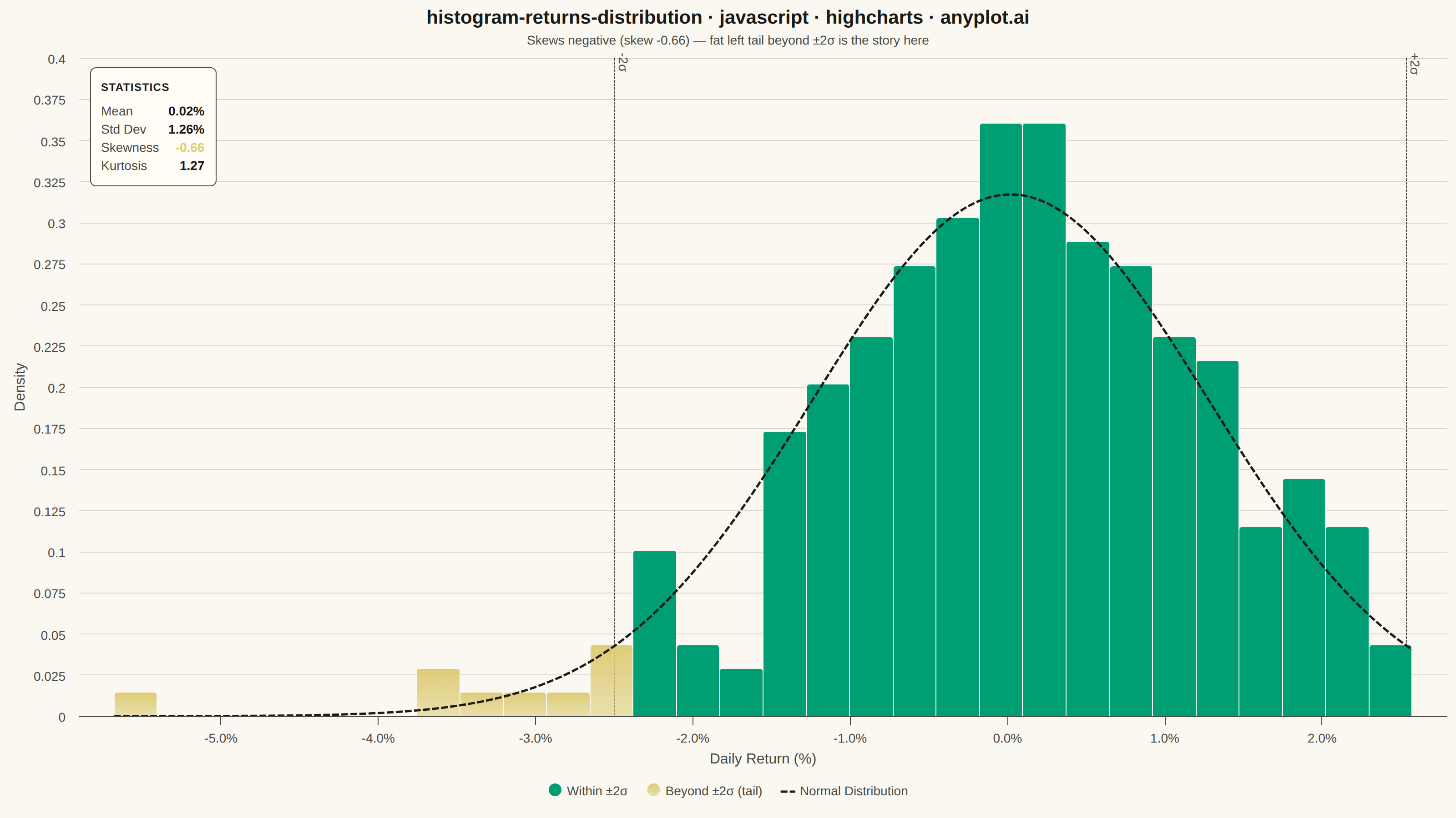
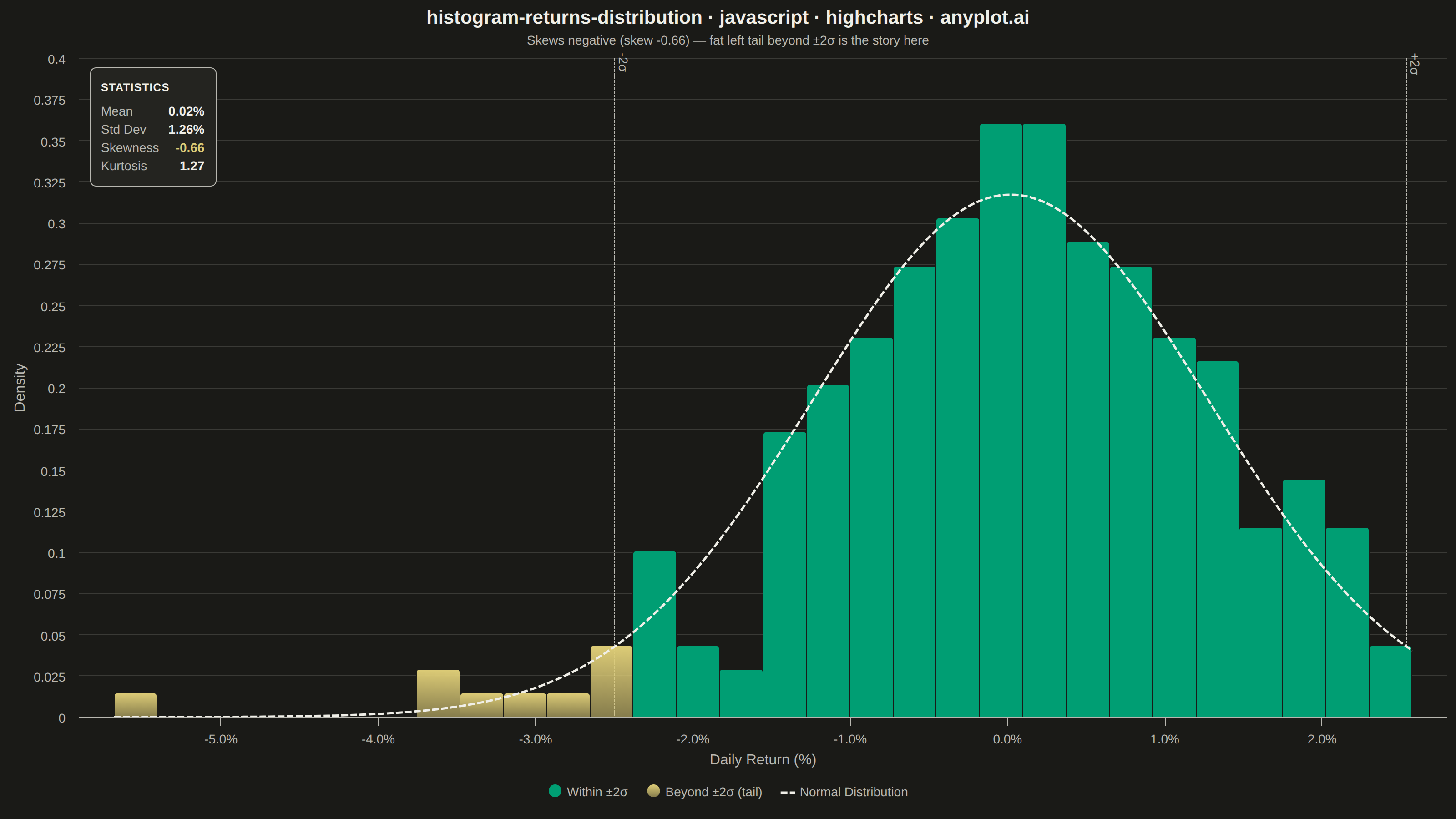
A histogram showing the distribution of financial returns (daily, weekly, or monthly) with a normal distribution overlay for comparison. This visualization is essential for risk analysis, allowing analysts to assess whether returns follow a normal distribution, identify fat tails indicating higher-than-expected extreme events, and measure asymmetry through skewness. Key statistics are displayed directly on the plot for quick interpretation.
// anyplot.ai
// histogram-returns-distribution: Returns Distribution Histogram
// Library: highcharts 12.6.0 | JavaScript 22.23.2
// Quality: 92/100 | Created: 2026-09-02

const t = window.ANYPLOT_TOKENS;

// --- Data (in-memory, deterministic LCG) ------------------------------------
function makeLcg(seed) {
  let state = seed >>> 0;
  return function () {
    state = (Math.imul(1103515245, state) + 12345) >>> 0;
    return state / 4294967296;
  };
}
const rand = makeLcg(20260215);

// Small math helpers (LCG sampler + normal PDF) are kept top-level since they
// are pure functions reused by both the data generation and the fitted-curve
// section below — inlining them would duplicate the Box-Muller/PDF formulas.
function randNormal() {
  const u1 = Math.max(rand(), 1e-9);
  const u2 = rand();
  return Math.sqrt(-2 * Math.log(u1)) * Math.cos(2 * Math.PI * u2);
}

const nObs = 252; // one trading year of daily returns
const muDaily = 0.04; // % drift
const sigmaDaily = 1.1; // % daily vol
const returns = [];
for (let i = 0; i < nObs; i++) {
  let z = randNormal();
  if (i % 23 === 0) z -= 1.8; // rare drawdown days -> negative skew, fat left tail
  if (i % 41 === 0) z += 1.3; // rare rally days
  returns.push(muDaily + sigmaDaily * z);
}

// --- Sample statistics --------------------------------------------------
const mean = returns.reduce((a, b) => a + b, 0) / nObs;
const m2 = returns.reduce((a, b) => a + (b - mean) ** 2, 0) / nObs;
const std = Math.sqrt((returns.reduce((a, b) => a + (b - mean) ** 2, 0)) / (nObs - 1));
const m3 = returns.reduce((a, b) => a + (b - mean) ** 3, 0) / nObs;
const m4 = returns.reduce((a, b) => a + (b - mean) ** 4, 0) / nObs;
const skewness = m3 / Math.pow(m2, 1.5);
const kurtosis = m4 / (m2 * m2) - 3; // excess kurtosis

// --- Histogram (density-normalized) --------------------------------------
const binCount = 30;
const minR = Math.min(...returns);
const maxR = Math.max(...returns);
const binWidth = (maxR - minR) / binCount;
const counts = new Array(binCount).fill(0);
returns.forEach((r) => {
  let idx = Math.floor((r - minR) / binWidth);
  if (idx >= binCount) idx = binCount - 1;
  if (idx < 0) idx = 0;
  counts[idx]++;
});
const density = counts.map((c) => c / (nObs * binWidth));
const binCenters = density.map((_, i) => minR + (i + 0.5) * binWidth);

const tailLo = mean - 2 * std;
const tailHi = mean + 2 * std;
const bodyData = [];
const tailData = [];
binCenters.forEach((c, i) => {
  if (c < tailLo || c > tailHi) {
    tailData.push({ x: c, y: density[i] });
    bodyData.push({ x: c, y: null });
  } else {
    bodyData.push({ x: c, y: density[i] });
    tailData.push({ x: c, y: null });
  }
});

// --- Fitted normal distribution curve ------------------------------------
function normalPdf(x, mu, sigma) {
  return Math.exp(-0.5 * ((x - mu) / sigma) ** 2) / (sigma * Math.sqrt(2 * Math.PI));
}
const curvePoints = 100;
const curveData = [];
for (let i = 0; i <= curvePoints; i++) {
  const x = minR + (i / curvePoints) * (maxR - minR);
  curveData.push([x, normalPdf(x, mean, std)]);
}

// --- Chart -------------------------------------------------------------
const title = "histogram-returns-distribution · javascript · highcharts · anyplot.ai";
const tailSide = skewness < 0 ? "left" : "right";
const subtitle =
  "Skews " + (skewness < 0 ? "negative" : "positive") + " (skew " + skewness.toFixed(2) +
  ") — fat " + tailSide + " tail beyond ±2σ is the story here";

Highcharts.chart("container", {
  chart: {
    type: "column",
    backgroundColor: "transparent",
    animation: false,
    style: { fontFamily: "inherit" },
    events: {
      load: function () {
        const chart = this;
        const row = (label, value, valueColor) =>
          '<div style="display:flex;justify-content:space-between;gap:18px;">' +
          '<span style="color:' + t.inkSoft + ';">' + label + "</span>" +
          '<b style="color:' + (valueColor || t.ink) + ';">' + value + "</b></div>";
        const statsText =
          '<div style="font-weight:700;font-size:12px;letter-spacing:0.06em;' +
          'text-transform:uppercase;color:' + t.ink + ';margin-bottom:6px;">Statistics</div>' +
          row("Mean", mean.toFixed(2) + "%") +
          row("Std Dev", std.toFixed(2) + "%") +
          row("Skewness", skewness.toFixed(2), t.amber) +
          row("Kurtosis", kurtosis.toFixed(2));
        chart.renderer
          .label(statsText, chart.plotLeft + 12, chart.plotTop + 10, undefined, undefined, undefined, true)
          .css({ color: t.inkSoft, fontSize: "14px", lineHeight: "20px" })
          .attr({
            fill: t.elevatedBg,
            stroke: t.inkSoft,
            "stroke-width": 1,
            padding: 12,
            r: 6,
            zIndex: 5,
            shadow: { color: "#000000", offsetX: 0, offsetY: 2, opacity: 0.18, width: 6 },
          })
          .add();
      },
    },
  },
  credits: { enabled: false },
  colors: t.palette,
  title: { text: title, style: { color: t.ink, fontSize: "21px", fontWeight: "600" } },
  subtitle: { text: subtitle, style: { color: t.inkSoft, fontSize: "14px" } },
  xAxis: {
    title: { text: "Daily Return (%)", style: { color: t.inkSoft, fontSize: "16px" } },
    lineColor: t.inkSoft,
    tickColor: t.inkSoft,
    gridLineColor: t.grid,
    labels: { style: { color: t.inkSoft, fontSize: "14px" }, format: "{value:.1f}%" },
    plotLines: [
      {
        value: tailLo,
        color: t.inkSoft,
        dashStyle: "ShortDash",
        width: 1,
        label: { text: "-2σ", style: { color: t.inkSoft, fontSize: "14px" }, y: -6 },
      },
      {
        value: tailHi,
        color: t.inkSoft,
        dashStyle: "ShortDash",
        width: 1,
        label: { text: "+2σ", style: { color: t.inkSoft, fontSize: "14px" }, y: -6 },
      },
    ],
  },
  yAxis: {
    title: { text: "Density", style: { color: t.inkSoft, fontSize: "16px" } },
    gridLineColor: t.grid,
    labels: { style: { color: t.inkSoft, fontSize: "14px" } },
  },
  legend: {
    itemStyle: { color: t.inkSoft, fontSize: "14px" },
    itemHoverStyle: { color: t.ink },
  },
  plotOptions: {
    column: {
      pointPadding: 0,
      groupPadding: 0,
      grouping: false,
      borderWidth: 1,
      borderColor: t.pageBg,
      pointRange: binWidth,
      animation: false,
    },
    series: { animation: false },
  },
  series: [
    { name: "Within ±2σ", type: "column", data: bodyData, color: t.palette[0] },
    {
      name: "Beyond ±2σ (tail)",
      type: "column",
      data: tailData,
      color: {
        linearGradient: { x1: 0, y1: 0, x2: 0, y2: 1 },
        stops: [
          [0, t.amber],
          [1, Highcharts.color(t.amber).setOpacity(0.55).get("rgba")],
        ],
      },
    },
    {
      name: "Normal Distribution",
      type: "spline",
      data: curveData,
      color: t.ink,
      dashStyle: "ShortDash",
      lineWidth: 2.5,
      marker: { enabled: false },
    },
  ],
});
Runnable source as JSON, for any HTTP client: https://api.anyplot.ai/specs/histogram-returns-distribution/highcharts/code. Any spec id and library id listed in llms-full.txt fit the same URL shape; every URL below is complete and callable.
{
  "spec_id": "histogram-returns-distribution",
  "language": "javascript",
  "library": "highcharts",
  "page": "https://anyplot.ai/histogram-returns-distribution/javascript/highcharts",
  "hub": "https://anyplot.ai/histogram-returns-distribution",
  "code_json": "https://api.anyplot.ai/specs/histogram-returns-distribution/highcharts/code",
  "spec_json": "https://api.anyplot.ai/specs/histogram-returns-distribution",
  "render_light_png": "https://storage.googleapis.com/anyplot-images/plots/histogram-returns-distribution/javascript/highcharts/plot-light.png",
  "render_dark_png": "https://storage.googleapis.com/anyplot-images/plots/histogram-returns-distribution/javascript/highcharts/plot-dark.png",
  "interactive_light_html": "https://storage.googleapis.com/anyplot-images/plots/histogram-returns-distribution/javascript/highcharts/plot-light.html",
  "interactive_dark_html": "https://storage.googleapis.com/anyplot-images/plots/histogram-returns-distribution/javascript/highcharts/plot-dark.html",
  "quality_score": 92.0,
  "license": "MIT",
  "guide": "https://anyplot.ai/llms.txt"
}
Part of Returns Distribution Histogram on anyplot.ai.