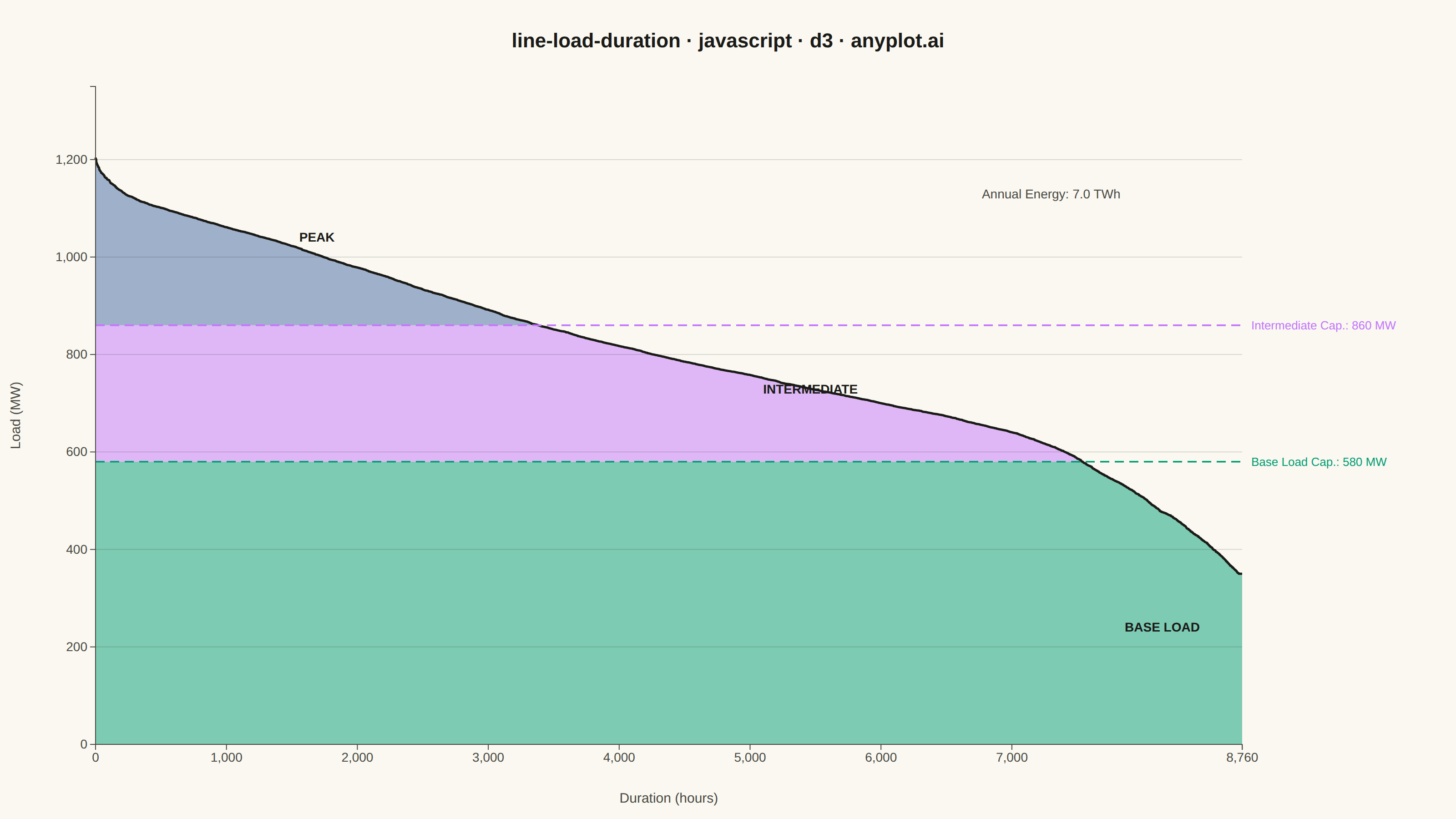
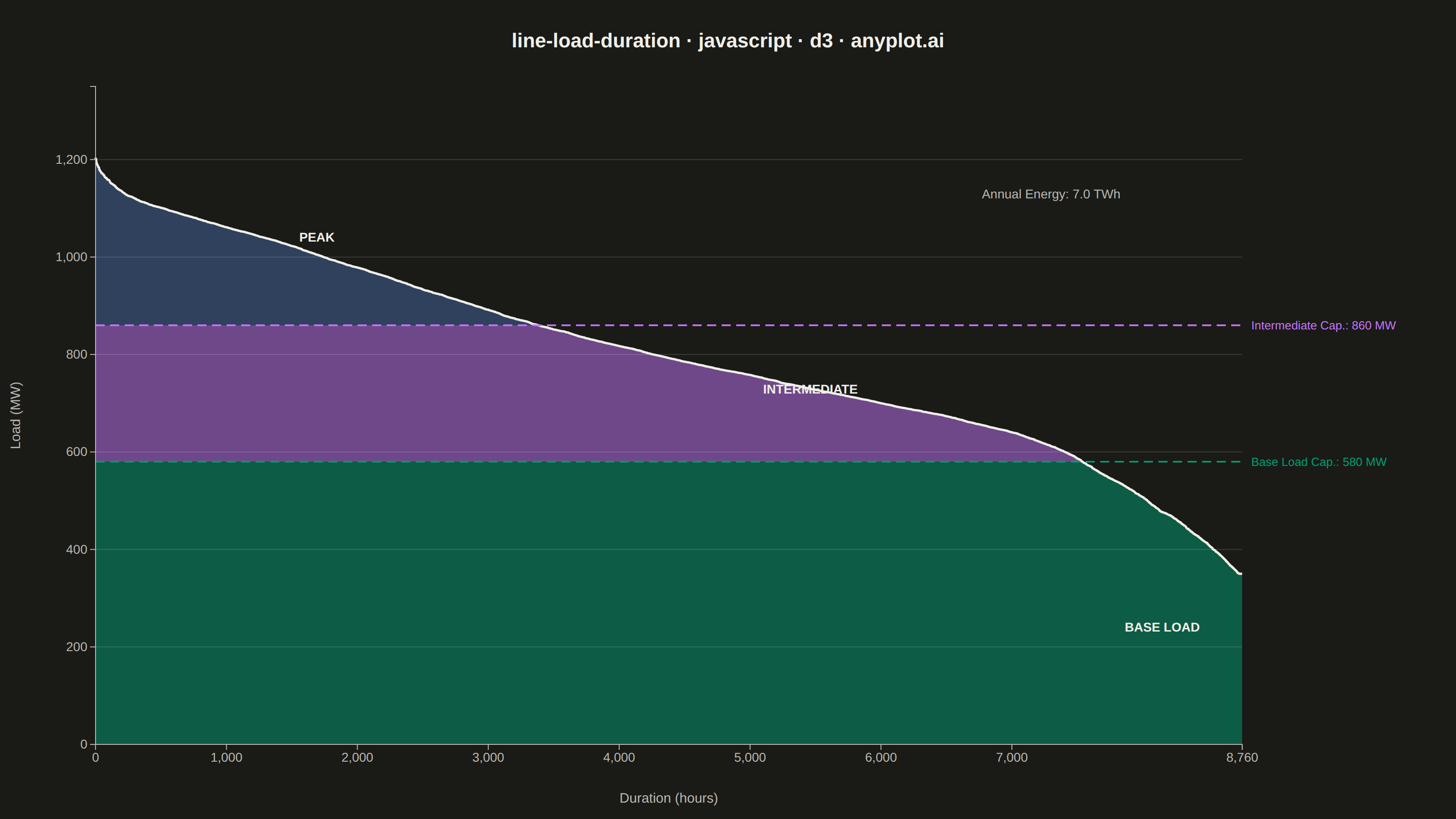
The same plot in 14 other libraries — JavaScript: Chart.js, Apache ECharts, Highcharts, MUI X Charts; Python: Altair, Bokeh, lets-plot, Matplotlib, Plotly, plotnine, Pygal, Seaborn; R: ggplot2; Julia: Makie.jl. Compare all 15 side by side: Load Duration Curve for Energy Systems in Python, R, Julia and JavaScript.
A load duration curve displays electrical power demand (MW) sorted from highest to lowest across all hours of a year (8,760 hours), forming a monotonically decreasing curve. It is a fundamental tool in power system planning, revealing the proportion of time that load exceeds a given level. The curve naturally segments into peak, intermediate, and base load regions, helping utilities determine the optimal generation capacity mix. The area under the curve represents total annual energy consumption.
// anyplot.ai
// line-load-duration: Load Duration Curve for Energy Systems
// Library: d3 7.9.0 | JavaScript 22.22.3
// Quality: 92/100 | Created: 2026-06-10
//# anyplot-orientation: landscape

const t = window.ANYPLOT_TOKENS;
const { width, height } = window.ANYPLOT_SIZE;

const margin = { top: 95, right: 235, bottom: 82, left: 105 };
const iw = width - margin.left - margin.right;
const ih = height - margin.top - margin.bottom;

// Deterministic LCG — no Math.random() in the browser harness
let seed = 42;
const lcg = () => {
  seed = (seed * 1664525 + 1013904223) >>> 0;
  return seed / 4294967296;
};

// Synthesize 8 760 hourly loads with seasonal + daily patterns, then sort descending
const raw = [];
for (let i = 0; i < 8760; i++) {
  const doy = Math.floor(i / 24);
  const hod = i % 24;
  const seasonal = 220 * Math.cos((doy / 365) * 2 * Math.PI);
  const daily = -150 * Math.cos((hod / 24) * 2 * Math.PI)
              - 80  * Math.cos((hod / 24) * 4 * Math.PI - 0.5);
  raw.push(800 + seasonal + daily + (lcg() - 0.5) * 80);
}
raw.sort((a, b) => b - a);

const data = raw.map((v, i) => ({
  hour: i,
  load_mw: Math.max(350, Math.min(1250, v)),
}));

// Capacity thresholds (MW) and statistics
const baseCap  = 580;
const interCap = 860;
const peakMax  = d3.max(data, d => d.load_mw);
const totalTWh = (data.reduce((s, d) => s + d.load_mw, 0) / 1e6).toFixed(1);

// Boundary indices (hours at which the curve crosses each threshold)
const peakEnd  = data.filter(d => d.load_mw > interCap).length;
const interEnd = data.filter(d => d.load_mw > baseCap).length;

// SVG scaffold
const svg = d3.select("#container").append("svg")
  .attr("width", width).attr("height", height);
const g = svg.append("g")
  .attr("transform", `translate(${margin.left},${margin.top})`);

// Scales
const x = d3.scaleLinear().domain([0, 8759]).range([0, iw]);
const y = d3.scaleLinear().domain([0, 1350]).range([ih, 0]);

// Area generators for three load regions (Imprint palette positions 0 → 2)
const areaBase = d3.area()
  .x(d => x(d.hour))
  .y0(y(0))
  .y1(d => y(Math.min(d.load_mw, baseCap)));

const areaInter = d3.area()
  .x(d => x(d.hour))
  .y0(y(baseCap))
  .y1(d => y(Math.min(d.load_mw, interCap)))
  .defined(d => d.load_mw > baseCap);

const areaPeak = d3.area()
  .x(d => x(d.hour))
  .y0(y(interCap))
  .y1(d => y(d.load_mw))
  .defined(d => d.load_mw > interCap);

// Filled regions
g.append("path").datum(data).attr("d", areaBase)
  .attr("fill", t.palette[0]).attr("fill-opacity", 0.50);
g.append("path").datum(data).attr("d", areaInter)
  .attr("fill", t.palette[1]).attr("fill-opacity", 0.50);
g.append("path").datum(data).attr("d", areaPeak)
  .attr("fill", t.palette[2]).attr("fill-opacity", 0.50);

// Horizontal gridlines (y-axis only, drawn on top of fills so they read through)
const gridG = g.append("g");
gridG.call(d3.axisLeft(y).ticks(7).tickSize(-iw).tickFormat(""));
gridG.select(".domain").remove();
gridG.selectAll(".tick line").attr("stroke", t.grid);

// LDC curve
g.append("path").datum(data)
  .attr("d", d3.line().x(d => x(d.hour)).y(d => y(d.load_mw)))
  .attr("fill", "none")
  .attr("stroke", t.ink)
  .attr("stroke-width", 2.5);

// Capacity reference lines (dashed, color-matched to their region)
[
  [baseCap,  "Base Load Cap.",    t.palette[0]],
  [interCap, "Intermediate Cap.", t.palette[1]],
].forEach(([cap, label, color]) => {
  g.append("line")
    .attr("x1", 0).attr("x2", iw)
    .attr("y1", y(cap)).attr("y2", y(cap))
    .attr("stroke", color).attr("stroke-width", 1.8)
    .attr("stroke-dasharray", "10,6");

  g.append("text")
    .attr("x", iw + 10).attr("y", y(cap)).attr("dy", "0.35em")
    .attr("fill", color)
    .style("font-size", "13px").style("font-weight", "500")
    .text(`${label}: ${cap} MW`);
});

// Axes
const xAx = g.append("g").attr("transform", `translate(0,${ih})`)
  .call(d3.axisBottom(x)
    .tickValues([0, 1000, 2000, 3000, 4000, 5000, 6000, 7000, 8760])
    .tickFormat(d3.format(",d")));

const yAx = g.append("g").call(d3.axisLeft(y).ticks(7));

[xAx, yAx].forEach(ax => {
  ax.selectAll("text").attr("fill", t.inkSoft).style("font-size", "14px");
  ax.selectAll(".tick line").attr("stroke", t.inkSoft);
  ax.select(".domain").attr("stroke", t.inkSoft);
});

// Axis labels
svg.append("text")
  .attr("x", margin.left + iw / 2).attr("y", height - 18)
  .attr("text-anchor", "middle")
  .attr("fill", t.inkSoft).style("font-size", "15px")
  .text("Duration (hours)");

svg.append("text")
  .attr("transform", `translate(22,${margin.top + ih / 2})rotate(-90)`)
  .attr("text-anchor", "middle")
  .attr("fill", t.inkSoft).style("font-size", "15px")
  .text("Load (MW)");

// Region labels (directly on the chart)
g.append("text")
  .attr("x", x(peakEnd / 2))
  .attr("y", y((interCap + peakMax) / 2))
  .attr("text-anchor", "middle")
  .attr("fill", t.ink).style("font-size", "14px").style("font-weight", "700")
  .text("PEAK");

g.append("text")
  .attr("x", x((peakEnd + interEnd) / 2))
  .attr("y", y((baseCap + interCap) / 2))
  .attr("text-anchor", "middle")
  .attr("fill", t.ink).style("font-size", "14px").style("font-weight", "700")
  .text("INTERMEDIATE");

g.append("text")
  .attr("x", x((interEnd + 8759) / 2))
  .attr("y", y(baseCap * 0.40))
  .attr("text-anchor", "middle")
  .attr("fill", t.ink).style("font-size", "14px").style("font-weight", "700")
  .text("BASE LOAD");

// Total energy annotation in upper-right empty space
g.append("text")
  .attr("x", x(7300)).attr("y", y(1120))
  .attr("text-anchor", "middle")
  .attr("fill", t.inkSoft).style("font-size", "14px")
  .text(`Annual Energy: ${totalTWh} TWh`);

// Title
svg.append("text")
  .attr("x", width / 2).attr("y", 52)
  .attr("text-anchor", "middle")
  .attr("fill", t.ink).style("font-size", "22px").style("font-weight", "600")
  .text("line-load-duration · javascript · d3 · anyplot.ai");
Runnable source as JSON, for any HTTP client: https://api.anyplot.ai/specs/line-load-duration/d3/code. Any spec id and library id listed in llms-full.txt fit the same URL shape; every URL below is complete and callable.
{
  "spec_id": "line-load-duration",
  "language": "javascript",
  "library": "d3",
  "page": "https://anyplot.ai/line-load-duration/javascript/d3",
  "hub": "https://anyplot.ai/line-load-duration",
  "code_json": "https://api.anyplot.ai/specs/line-load-duration/d3/code",
  "spec_json": "https://api.anyplot.ai/specs/line-load-duration",
  "render_light_png": "https://storage.googleapis.com/anyplot-images/plots/line-load-duration/javascript/d3/plot-light.png",
  "render_dark_png": "https://storage.googleapis.com/anyplot-images/plots/line-load-duration/javascript/d3/plot-dark.png",
  "interactive_light_html": "https://storage.googleapis.com/anyplot-images/plots/line-load-duration/javascript/d3/plot-light.html",
  "interactive_dark_html": "https://storage.googleapis.com/anyplot-images/plots/line-load-duration/javascript/d3/plot-dark.html",
  "quality_score": 92.0,
  "license": "MIT",
  "guide": "https://anyplot.ai/llms.txt"
}
Part of Load Duration Curve for Energy Systems on anyplot.ai.