The same plot in 14 other libraries — JavaScript: Chart.js, D3.js, Apache ECharts, Highcharts; Python: Altair, Bokeh, lets-plot, Matplotlib, Plotly, plotnine, Pygal, Seaborn; R: ggplot2; Julia: Makie.jl. Compare all 15 side by side: Load Duration Curve for Energy Systems in Python, R, Julia and JavaScript.
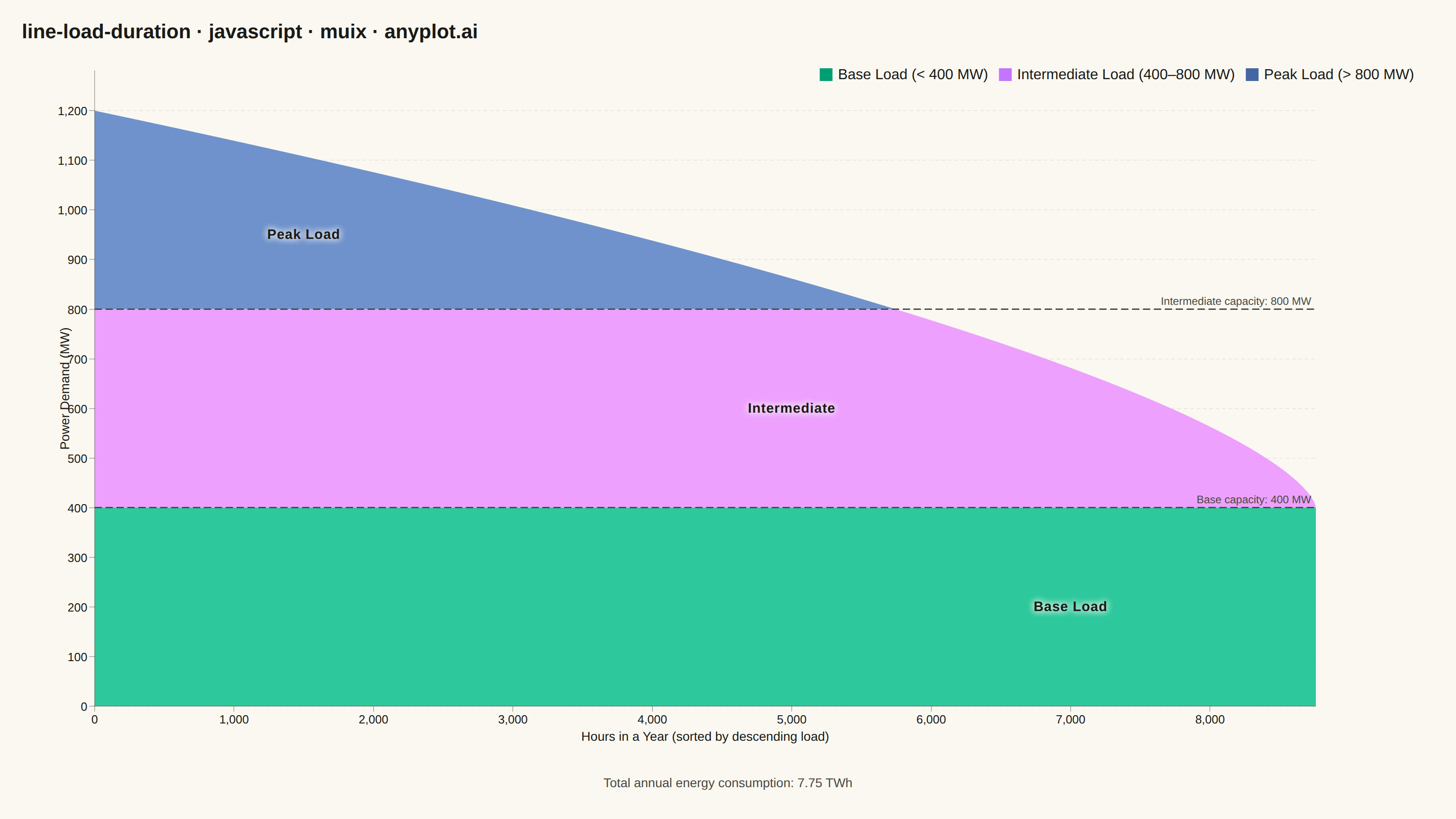
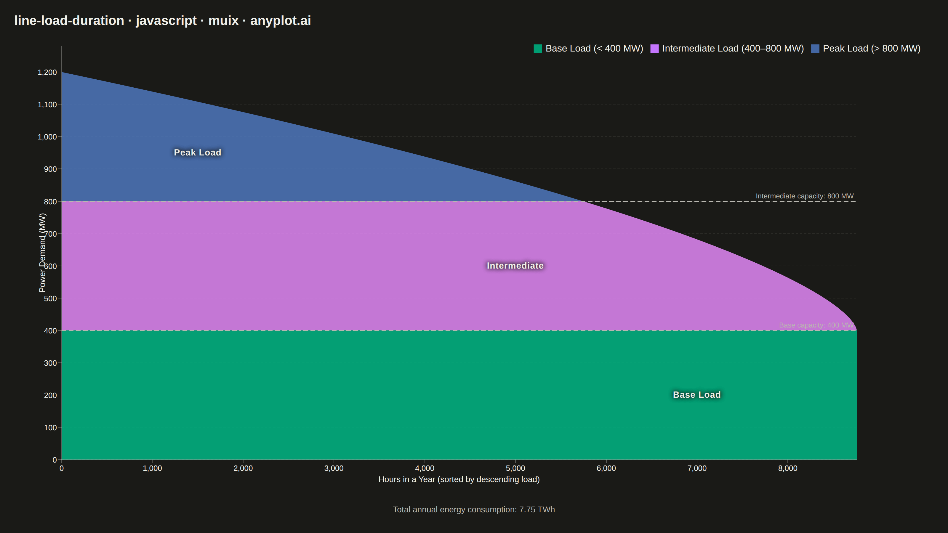
A load duration curve displays electrical power demand (MW) sorted from highest to lowest across all hours of a year (8,760 hours), forming a monotonically decreasing curve. It is a fundamental tool in power system planning, revealing the proportion of time that load exceeds a given level. The curve naturally segments into peak, intermediate, and base load regions, helping utilities determine the optimal generation capacity mix. The area under the curve represents total annual energy consumption.
// anyplot.ai
// line-load-duration: Load Duration Curve for Energy Systems
// Library: muix 7.29.1 | JavaScript 22.22.3
// Quality: 88/100 | Created: 2026-06-10
import { LineChart } from "@mui/x-charts/LineChart";
import { ChartsReferenceLine } from "@mui/x-charts/ChartsReferenceLine";

const t = window.ANYPLOT_TOKENS;

// --- Data (deterministic, no RNG) -------------------------------------------
// 8,760 hours sorted descending: peak ≈ 1200 MW → base ≈ 400 MW
const N_HOURS = 8760;
const hours = Array.from({ length: N_HOURS }, (_, i) => i);

// Power-law decay gives realistic LDC shape (steep peak drop, flat base tail)
const loadMW = hours.map(h => 400 + 800 * Math.pow(1 - h / (N_HOURS - 1), 0.65));

// Decompose into three stacked bands
const baseData  = hours.map(() => 400);
const interData = hours.map(h => Math.min(Math.max(loadMW[h] - 400, 0), 400));
const peakData  = hours.map(h => Math.max(loadMW[h] - 800, 0));

const totalEnergyTWh = (loadMW.reduce((s, v) => s + v, 0) / 1e6).toFixed(2);

const TITLE = "line-load-duration · javascript · muix · anyplot.ai";

// Chart margins — declared once, shared by LineChart and the annotation overlay
const MARGIN = { top: 20, right: 130, bottom: 72, left: 80 };
const Y_MAX = 1280;
const X_MAX = N_HOURS - 1;

// Convert data-space coordinates to CSS px within the chart container
function toPixel(x, y, cW, cH) {
  const dw = cW - MARGIN.left - MARGIN.right;
  const dh = cH - MARGIN.top - MARGIN.bottom;
  return {
    left: MARGIN.left + (x / X_MAX) * dw,
    top:  MARGIN.top  + (1 - y / Y_MAX) * dh,
  };
}

// --- Component (default-exported; harness mounts it with no props) -----------
export default function Chart() {
  const W = window.ANYPLOT_SIZE.width;
  const H = window.ANYPLOT_SIZE.height;

  const HEADER_H = 50;
  const FOOTER_H = 28;
  const PAD_TOP  = 20;
  const PAD_BOT  = 12;
  const PAD_H    = 48;
  const chartW   = W - PAD_H;
  const chartH   = H - PAD_TOP - HEADER_H - FOOTER_H - PAD_BOT;

  // Labels placed at representative (x, y) data coords inside each band
  // Base band: 0–400 MW (y=200 at x=7000 → far-right flat region)
  // Intermediate band: 400–800 MW (y=600 at x=5000 → saturated mid-band)
  // Peak band: >800 MW (y=950 at x=1500 → steep left portion)
  const bandLabels = [
    { x: 7000, y: 200, text: "Base Load"    },
    { x: 5000, y: 600, text: "Intermediate" },
    { x: 1500, y: 950, text: "Peak Load"    },
  ];

  return (
    <div style={{
      width: W,
      height: H,
      backgroundColor: t.pageBg,
      display: "flex",
      flexDirection: "column",
      padding: `${PAD_TOP}px 24px ${PAD_BOT}px`,
      boxSizing: "border-box",
      fontFamily: "sans-serif",
    }}>
      {/* Chart title */}
      <div style={{
        color: t.ink,
        fontSize: 22,
        fontWeight: 600,
        lineHeight: "30px",
        marginBottom: 8,
        flexShrink: 0,
      }}>
        {TITLE}
      </div>

      {/* Stacked-area chart with region-label overlay */}
      <div style={{ position: "relative", width: chartW, height: chartH, flexShrink: 0 }}>
        <LineChart
          width={chartW}
          height={chartH}
          margin={MARGIN}
          skipAnimation
          grid={{ horizontal: true }}
          colors={[t.palette[0], t.palette[1], t.palette[2]]}
          xAxis={[{
            data: hours,
            label: "Hours in a Year (sorted by descending load)",
            min: 0,
            max: X_MAX,
            tickInterval: [0, 1000, 2000, 3000, 4000, 5000, 6000, 7000, 8000],
            tickLabelStyle: { fontSize: 13 },
          }]}
          yAxis={[{
            label: "Power Demand (MW)",
            min: 0,
            max: Y_MAX,
            tickLabelStyle: { fontSize: 13 },
          }]}
          series={[
            {
              data: baseData,
              area: true,
              stack: "load",
              label: "Base Load (< 400 MW)",
              showMark: false,
              curve: "linear",
            },
            {
              data: interData,
              area: true,
              stack: "load",
              label: "Intermediate Load (400–800 MW)",
              showMark: false,
              curve: "linear",
            },
            {
              data: peakData,
              area: true,
              stack: "load",
              label: "Peak Load (> 800 MW)",
              showMark: false,
              curve: "linear",
            },
          ]}
          sx={{
            "& .MuiLineElement-root":  { strokeWidth: 0 },
            "& .MuiAreaElement-root":  { fillOpacity: 0.82 },
            "& .MuiChartsGrid-line":   { stroke: t.grid, strokeOpacity: 0.5, strokeDasharray: "4 3" },
            "& .MuiChartsAxis-line":   { stroke: t.inkSoft, strokeOpacity: 0.3 },
            "& .MuiChartsAxis-tick":   { stroke: t.inkSoft, strokeOpacity: 0.3 },
          }}
          slotProps={{
            legend: {
              position: { vertical: "top", horizontal: "right" },
              itemMarkWidth: 14,
              itemMarkHeight: 14,
              markGap: 6,
              itemGap: 12,
            },
          }}
        >
          {/* Horizontal dashed lines at capacity tier boundaries */}
          <ChartsReferenceLine
            y={400}
            label="Base capacity: 400 MW"
            lineStyle={{ stroke: t.inkSoft, strokeDasharray: "8 4", strokeWidth: 1.5 }}
            labelStyle={{ fontSize: 12, fill: t.inkSoft }}
            labelAlign="end"
          />
          <ChartsReferenceLine
            y={800}
            label="Intermediate capacity: 800 MW"
            lineStyle={{ stroke: t.inkSoft, strokeDasharray: "8 4", strokeWidth: 1.5 }}
            labelStyle={{ fontSize: 12, fill: t.inkSoft }}
            labelAlign="end"
          />
        </LineChart>

        {/* Direct in-band region labels — spec requires labeling each band on the plot */}
        {bandLabels.map(({ x, y, text }) => {
          const pos = toPixel(x, y, chartW, chartH);
          return (
            <div
              key={text}
              style={{
                position: "absolute",
                left: pos.left,
                top: pos.top,
                transform: "translate(-50%, -50%)",
                color: t.ink,
                fontSize: 15,
                fontWeight: 700,
                fontFamily: "sans-serif",
                pointerEvents: "none",
                textShadow: `0 0 8px ${t.pageBg}, 0 0 8px ${t.pageBg}`,
                letterSpacing: "0.04em",
                whiteSpace: "nowrap",
              }}
            >
              {text}
            </div>
          );
        })}
      </div>

      {/* Total energy annotation */}
      <div style={{
        color: t.inkSoft,
        fontSize: 14,
        textAlign: "center",
        marginTop: 4,
        flexShrink: 0,
        fontFamily: "sans-serif",
      }}>
        Total annual energy consumption: {totalEnergyTWh} TWh
      </div>
    </div>
  );
}
Runnable source as JSON, for any HTTP client: https://api.anyplot.ai/specs/line-load-duration/muix/code. Any spec id and library id listed in llms-full.txt fit the same URL shape; every URL below is complete and callable.
{
  "spec_id": "line-load-duration",
  "language": "javascript",
  "library": "muix",
  "page": "https://anyplot.ai/line-load-duration/javascript/muix",
  "hub": "https://anyplot.ai/line-load-duration",
  "code_json": "https://api.anyplot.ai/specs/line-load-duration/muix/code",
  "spec_json": "https://api.anyplot.ai/specs/line-load-duration",
  "render_light_png": "https://storage.googleapis.com/anyplot-images/plots/line-load-duration/javascript/muix/plot-light.png",
  "render_dark_png": "https://storage.googleapis.com/anyplot-images/plots/line-load-duration/javascript/muix/plot-dark.png",
  "interactive_light_html": "https://storage.googleapis.com/anyplot-images/plots/line-load-duration/javascript/muix/plot-light.html",
  "interactive_dark_html": "https://storage.googleapis.com/anyplot-images/plots/line-load-duration/javascript/muix/plot-dark.html",
  "quality_score": 88.0,
  "license": "MIT",
  "guide": "https://anyplot.ai/llms.txt"
}
Part of Load Duration Curve for Energy Systems on anyplot.ai.