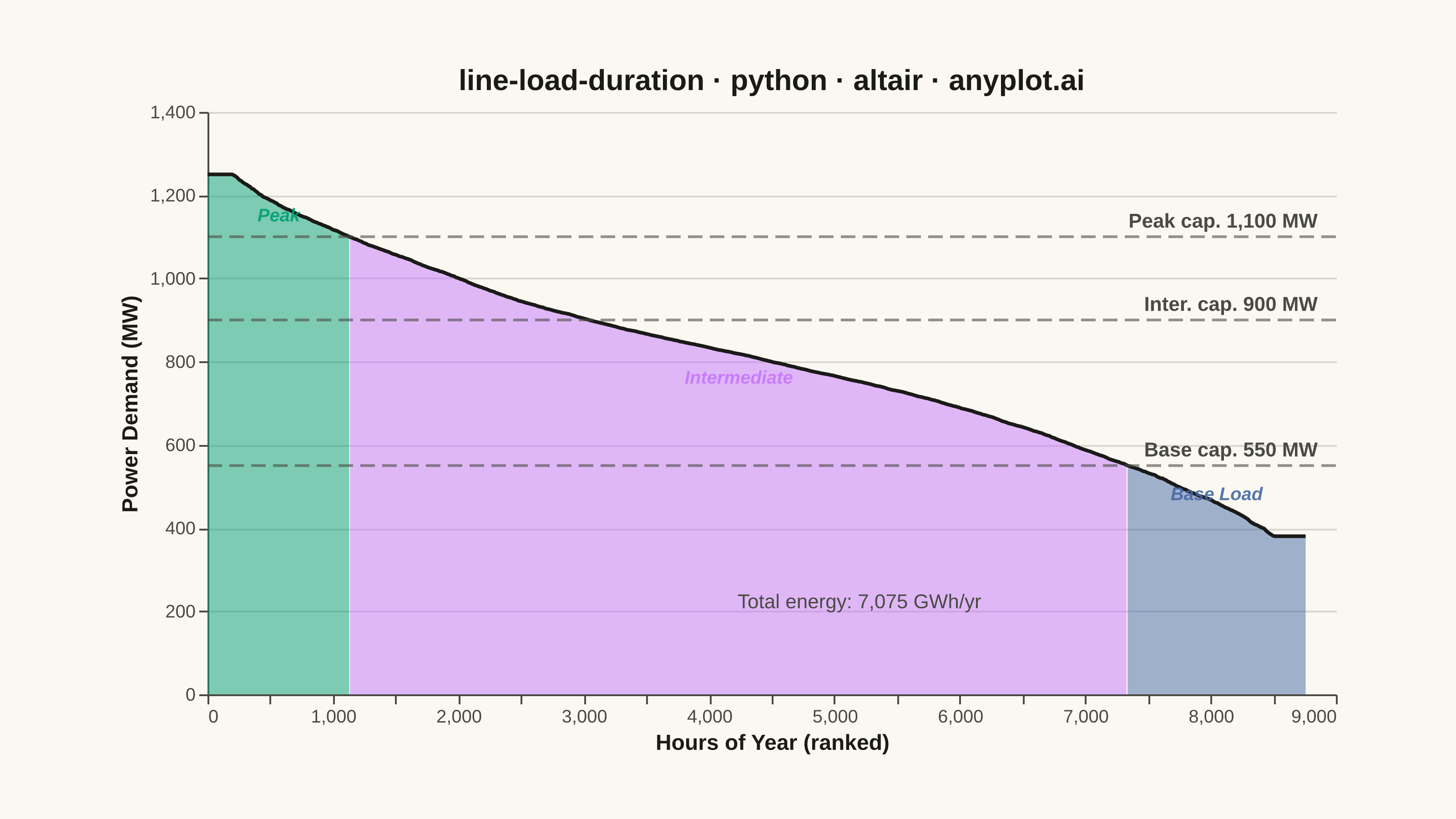
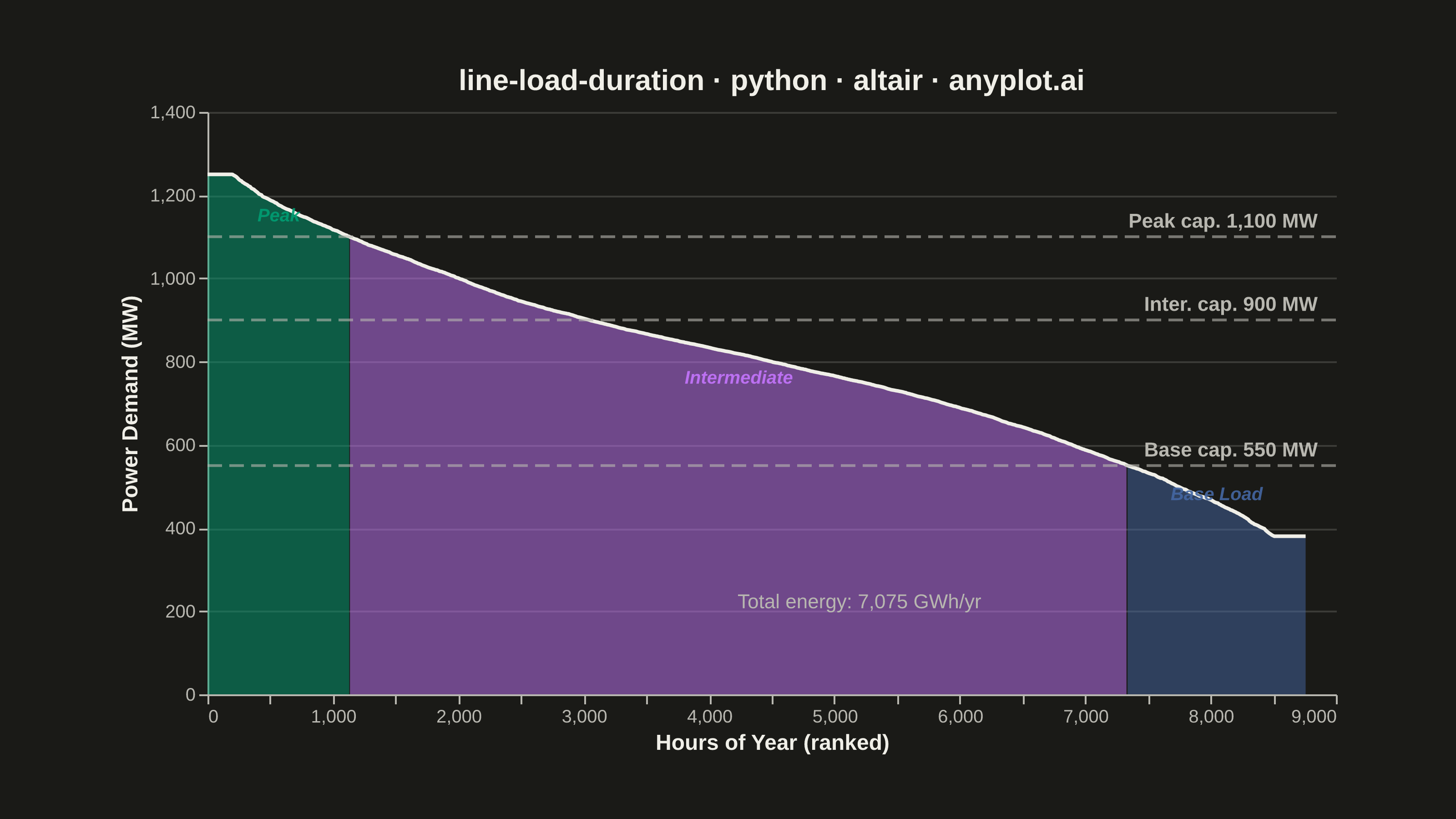
A load duration curve displays electrical power demand (MW) sorted from highest to lowest across all hours of a year (8,760 hours), forming a monotonically decreasing curve. It is a fundamental tool in power system planning, revealing the proportion of time that load exceeds a given level. The curve naturally segments into peak, intermediate, and base load regions, helping utilities determine the optimal generation capacity mix. The area under the curve represents total annual energy consumption.
""" anyplot.ai
line-load-duration: Load Duration Curve for Energy Systems
Library: altair 6.2.1 | Python 3.13.13
Quality: 88/100 | Updated: 2026-06-10
"""

import os
import sys


# Remove the script's own directory from sys.path so that `import altair`
# finds the installed package, not this file (which shares the library name).
_this_dir = os.path.dirname(os.path.abspath(__file__))
sys.path = [p for p in sys.path if os.path.abspath(p) != _this_dir]

import altair as alt
import numpy as np
import pandas as pd
from PIL import Image


# Theme-adaptive chrome — Imprint palette
THEME = os.getenv("ANYPLOT_THEME", "light")
PAGE_BG = "#FAF8F1" if THEME == "light" else "#1A1A17"
ELEVATED_BG = "#FFFDF6" if THEME == "light" else "#242420"
INK = "#1A1A17" if THEME == "light" else "#F0EFE8"
INK_SOFT = "#4A4A44" if THEME == "light" else "#B8B7B0"
INK_MUTED = "#6B6A63" if THEME == "light" else "#A8A79F"

# Imprint palette — load duration regions (positions 1–3)
PEAK_COLOR = "#009E73"  # position 1: brand green
INTER_COLOR = "#C475FD"  # position 2: lavender
BASE_COLOR = "#4467A3"  # position 3: blue

# ── Data ──────────────────────────────────────────────────────────────────────
np.random.seed(42)
HOURS = 8760
t = np.arange(HOURS)

load_mw = (
    400
    + 350
    + 200 * np.sin(2 * np.pi * (t % 24 - 6) / 24)
    + 250 * np.cos(2 * np.pi * (t / 24 - 30) / 365)
    + np.where((t // 24) % 7 < 5, 80, 0)
    + np.random.normal(0, 50, HOURS)
)
load_mw = np.clip(load_mw, 380, 1250)
load_sorted = np.sort(load_mw)[::-1]

PEAK_CAP = 1100
INTER_CAP = 900
BASE_CAP = 550

peak_end = int(np.searchsorted(-load_sorted, -PEAK_CAP))
inter_end = int(np.searchsorted(-load_sorted, -BASE_CAP))
total_gwh = np.trapezoid(load_sorted) / 1000

# Downsample 8760 → ~877 points for Vega performance
step = 10
idx = np.unique(np.append(np.arange(0, HOURS, step), HOURS - 1))
load_ds = load_sorted[idx]
hour_ds = idx.astype(float)

# Per-region DataFrames for coloured fills (non-overlapping in x)
pm = hour_ds <= peak_end
peak_df = pd.DataFrame({"hour": hour_ds[pm], "load_mw": load_ds[pm]})

im = (hour_ds >= peak_end) & (hour_ds <= inter_end)
inter_df = pd.DataFrame(
    {
        "hour": np.concatenate([[float(peak_end)], hour_ds[im]]),
        "load_mw": np.concatenate([[np.interp(peak_end, hour_ds, load_ds)], load_ds[im]]),
    }
)

bm = hour_ds >= inter_end
base_df = pd.DataFrame(
    {
        "hour": np.concatenate([[float(inter_end)], hour_ds[bm]]),
        "load_mw": np.concatenate([[np.interp(inter_end, hour_ds, load_ds)], load_ds[bm]]),
    }
)

full_df = pd.DataFrame({"hour": hour_ds, "load_mw": load_ds})

# ── Chart layers ──────────────────────────────────────────────────────────────
Y_DOM = alt.Scale(domain=[0, 1400])

peak_area = (
    alt.Chart(peak_df)
    .mark_area(opacity=0.5, color=PEAK_COLOR)
    .encode(x=alt.X("hour:Q"), y=alt.Y("load_mw:Q", scale=Y_DOM))
)
inter_area = (
    alt.Chart(inter_df)
    .mark_area(opacity=0.5, color=INTER_COLOR)
    .encode(x=alt.X("hour:Q"), y=alt.Y("load_mw:Q", scale=Y_DOM))
)
base_area = (
    alt.Chart(base_df)
    .mark_area(opacity=0.5, color=BASE_COLOR)
    .encode(x=alt.X("hour:Q"), y=alt.Y("load_mw:Q", scale=Y_DOM))
)

line = (
    alt.Chart(full_df)
    .mark_line(color=INK, strokeWidth=2.0)
    .encode(
        x=alt.X("hour:Q", title="Hours of Year (ranked)", axis=alt.Axis(format=",d")),
        y=alt.Y("load_mw:Q", title="Power Demand (MW)", scale=Y_DOM),
        tooltip=[
            alt.Tooltip("hour:Q", title="Hour Rank", format=",d"),
            alt.Tooltip("load_mw:Q", title="Load (MW)", format=",.0f"),
        ],
    )
)

# Horizontal dashed capacity tier lines
tier_df = pd.DataFrame(
    {"y": [PEAK_CAP, INTER_CAP, BASE_CAP], "label": ["Peak cap. 1,100 MW", "Inter. cap. 900 MW", "Base cap. 550 MW"]}
)
tier_rules = (
    alt.Chart(tier_df)
    .mark_rule(strokeDash=[8, 4], strokeWidth=1.5, opacity=0.6)
    .encode(y=alt.Y("y:Q", scale=Y_DOM), color=alt.value(INK_SOFT))
)
tier_labels = (
    alt.Chart(tier_df)
    .mark_text(align="right", dx=-4, dy=-8, fontSize=11, fontWeight="bold", color=INK_SOFT)
    .encode(x=alt.value(614), y=alt.Y("y:Q", scale=Y_DOM), text="label:N")
)

# Region identity labels inside each coloured fill
peak_lbl = (
    alt.Chart(pd.DataFrame({"hour": [peak_end / 2], "load_mw": [1150.0], "t": ["Peak"]}))
    .mark_text(fontSize=10, fontWeight="bold", fontStyle="italic", color=PEAK_COLOR, opacity=0.9)
    .encode(x="hour:Q", y=alt.Y("load_mw:Q", scale=Y_DOM), text="t:N")
)
inter_lbl = (
    alt.Chart(pd.DataFrame({"hour": [(peak_end + inter_end) / 2], "load_mw": [760.0], "t": ["Intermediate"]}))
    .mark_text(fontSize=10, fontWeight="bold", fontStyle="italic", color=INTER_COLOR, opacity=0.9)
    .encode(x="hour:Q", y=alt.Y("load_mw:Q", scale=Y_DOM), text="t:N")
)
base_lbl = (
    alt.Chart(pd.DataFrame({"hour": [(inter_end + HOURS) / 2], "load_mw": [480.0], "t": ["Base Load"]}))
    .mark_text(fontSize=10, fontWeight="bold", fontStyle="italic", color=BASE_COLOR, opacity=0.9)
    .encode(x="hour:Q", y=alt.Y("load_mw:Q", scale=Y_DOM), text="t:N")
)
energy_lbl = (
    alt.Chart(pd.DataFrame({"hour": [5200.0], "load_mw": [220.0], "t": [f"Total energy: {total_gwh:,.0f} GWh/yr"]}))
    .mark_text(fontSize=11, color=INK_SOFT)
    .encode(x="hour:Q", y=alt.Y("load_mw:Q", scale=Y_DOM), text="t:N")
)

# Crosshair selection for interactive HTML
nearest = alt.selection_point(nearest=True, on="pointerover", fields=["hour"], empty=False)
xhair_pt = (
    alt.Chart(full_df)
    .mark_point(size=80, color=INK, filled=True)
    .encode(x="hour:Q", y="load_mw:Q", opacity=alt.condition(nearest, alt.value(1), alt.value(0)))
    .add_params(nearest)
)
xhair_rule = (
    alt.Chart(full_df)
    .mark_rule(color=INK_SOFT, strokeDash=[4, 4], strokeWidth=1)
    .encode(x="hour:Q", opacity=alt.condition(nearest, alt.value(0.6), alt.value(0)))
)

TITLE = "line-load-duration · python · altair · anyplot.ai"
STATIC_LAYERS = [
    peak_area,
    inter_area,
    base_area,
    line,
    tier_rules,
    tier_labels,
    peak_lbl,
    inter_lbl,
    base_lbl,
    energy_lbl,
]

# ── PNG (static) ──────────────────────────────────────────────────────────────
chart = (
    alt.layer(*STATIC_LAYERS)
    .properties(width=620, height=320, background=PAGE_BG, title=alt.Title(TITLE, fontSize=16))
    .configure_view(fill=PAGE_BG, strokeWidth=0, continuousWidth=620, continuousHeight=320)
    .configure_axis(
        domainColor=INK_SOFT,
        tickColor=INK_SOFT,
        gridColor=INK,
        gridOpacity=0.15,
        labelColor=INK_SOFT,
        titleColor=INK,
        labelFontSize=10,
        titleFontSize=12,
    )
    .configure_axisX(grid=False)
    .configure_title(color=INK)
    .configure_legend(fillColor=ELEVATED_BG, strokeColor=INK_SOFT, labelColor=INK_SOFT, titleColor=INK)
)
chart.save(f"plot-{THEME}.png", scale_factor=4.0)

# Pad to exact 3200 × 1800 canvas (vl-convert inner view is smaller)
TW, TH = 3200, 1800
_img = Image.open(f"plot-{THEME}.png").convert("RGB")
_w, _h = _img.size
if _w > TW or _h > TH:
    raise SystemExit(
        f"altair vl-convert produced {_w}×{_h}, exceeds target {TW}×{TH}. "
        "Shrink chart .properties(width=, height=) and re-render."
    )
if _w < TW or _h < TH:
    _canvas = Image.new("RGB", (TW, TH), PAGE_BG)
    _canvas.paste(_img, ((TW - _w) // 2, (TH - _h) // 2))
    _canvas.save(f"plot-{THEME}.png")

# ── Interactive HTML ──────────────────────────────────────────────────────────
inter_chart = (
    alt.layer(*STATIC_LAYERS, xhair_pt, xhair_rule)
    .properties(width=620, height=320, background=PAGE_BG, title=alt.Title(TITLE, fontSize=16))
    .configure_view(fill=PAGE_BG, strokeWidth=0, continuousWidth=620, continuousHeight=320)
    .configure_axis(
        domainColor=INK_SOFT,
        tickColor=INK_SOFT,
        gridColor=INK,
        gridOpacity=0.15,
        labelColor=INK_SOFT,
        titleColor=INK,
        labelFontSize=10,
        titleFontSize=12,
    )
    .configure_axisX(grid=False)
    .configure_title(color=INK)
    .configure_legend(fillColor=ELEVATED_BG, strokeColor=INK_SOFT, labelColor=INK_SOFT, titleColor=INK)
    .interactive()
)
inter_chart.save(f"plot-{THEME}.html")
Runnable source as JSON, for any HTTP client: https://api.anyplot.ai/specs/line-load-duration/altair/code. Any spec id and library id listed in llms-full.txt fit the same URL shape; every URL below is complete and callable.
{
  "spec_id": "line-load-duration",
  "language": "python",
  "library": "altair",
  "page": "https://anyplot.ai/line-load-duration/python/altair",
  "hub": "https://anyplot.ai/line-load-duration",
  "code_json": "https://api.anyplot.ai/specs/line-load-duration/altair/code",
  "spec_json": "https://api.anyplot.ai/specs/line-load-duration",
  "render_light_png": "https://storage.googleapis.com/anyplot-images/plots/line-load-duration/python/altair/plot-light.png",
  "render_dark_png": "https://storage.googleapis.com/anyplot-images/plots/line-load-duration/python/altair/plot-dark.png",
  "interactive_light_html": "https://storage.googleapis.com/anyplot-images/plots/line-load-duration/python/altair/plot-light.html",
  "interactive_dark_html": "https://storage.googleapis.com/anyplot-images/plots/line-load-duration/python/altair/plot-dark.html",
  "quality_score": 88.0,
  "license": "MIT",
  "guide": "https://anyplot.ai/llms.txt"
}
Part of Load Duration Curve for Energy Systems on anyplot.ai.