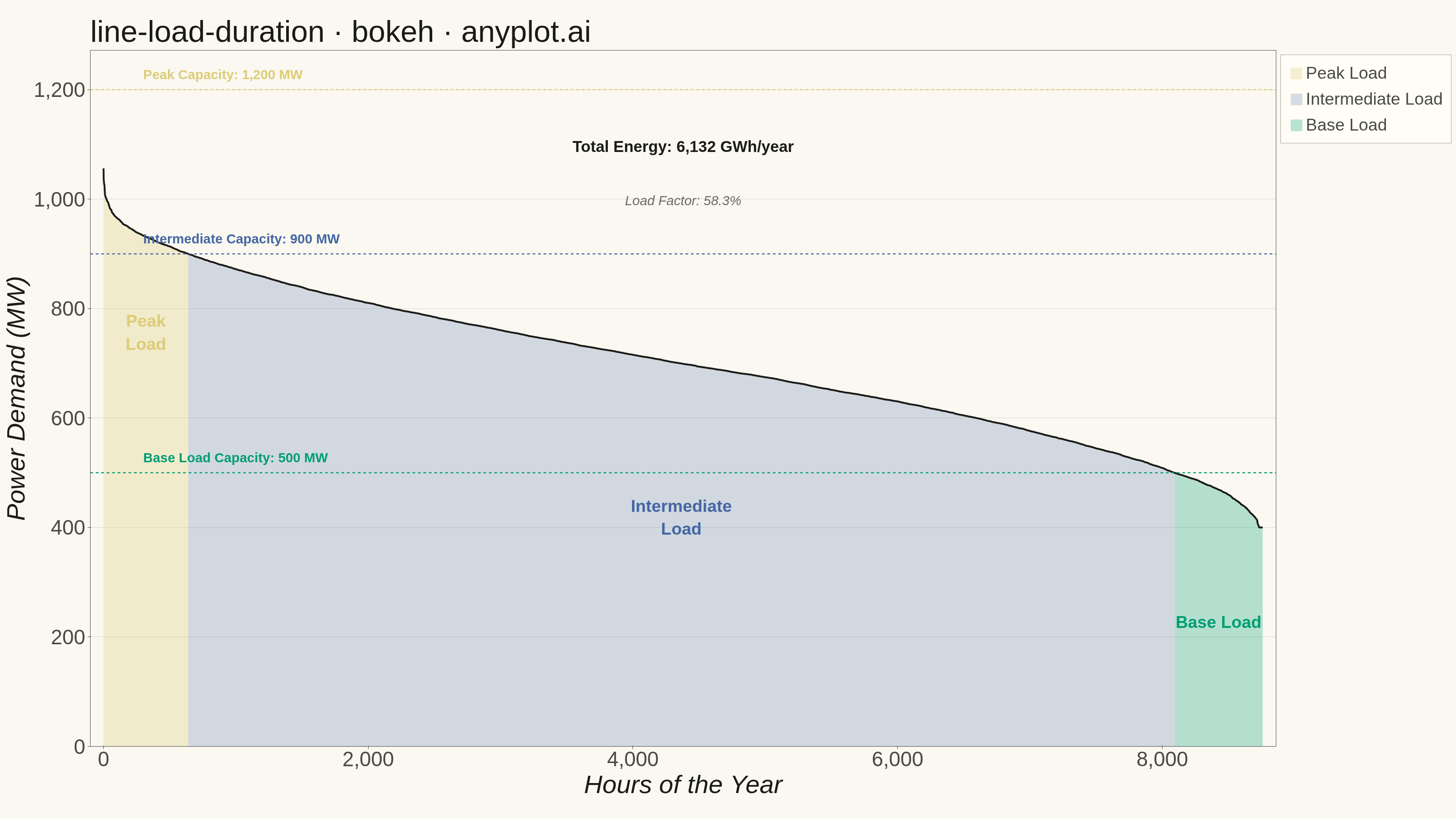
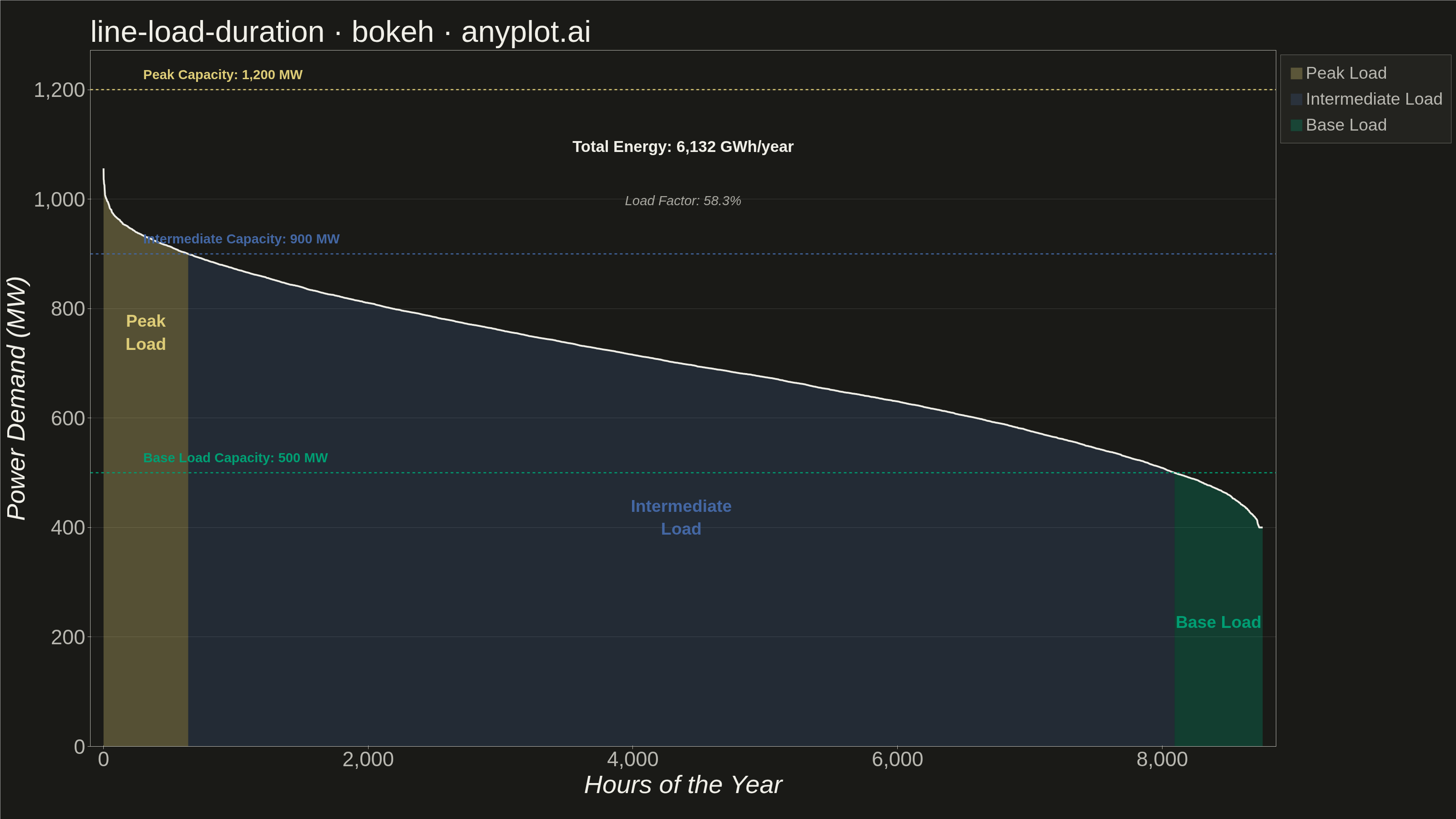
A load duration curve displays electrical power demand (MW) sorted from highest to lowest across all hours of a year (8,760 hours), forming a monotonically decreasing curve. It is a fundamental tool in power system planning, revealing the proportion of time that load exceeds a given level. The curve naturally segments into peak, intermediate, and base load regions, helping utilities determine the optimal generation capacity mix. The area under the curve represents total annual energy consumption.
""" anyplot.ai
line-load-duration: Load Duration Curve for Energy Systems
Library: bokeh 3.9.1 | Python 3.13.13
Quality: 90/100 | Updated: 2026-06-10
"""

import os
import sys
import time
from pathlib import Path


# Prevent this script from shadowing the installed bokeh package on sys.path
_script_dir = os.path.dirname(os.path.abspath(__file__))
if _script_dir in sys.path:
    sys.path.remove(_script_dir)

import numpy as np
from bokeh.io import output_file, save
from bokeh.models import ColumnDataSource, HoverTool, Label, Legend, NumeralTickFormatter, Span
from bokeh.plotting import figure
from selenium import webdriver
from selenium.webdriver.chrome.options import Options


# Theme
THEME = os.getenv("ANYPLOT_THEME", "light")

# Theme-adaptive chrome tokens (Imprint style guide)
PAGE_BG = "#FAF8F1" if THEME == "light" else "#1A1A17"
ELEVATED_BG = "#FFFDF6" if THEME == "light" else "#242420"
INK = "#1A1A17" if THEME == "light" else "#F0EFE8"
INK_SOFT = "#4A4A44" if THEME == "light" else "#B8B7B0"
INK_MUTED = "#6B6A63" if THEME == "light" else "#A8A79F"

# Imprint palette — semantic assignments for load regions
# Base Load  → brand green #009E73 (Imprint pos 1 — steady, reliable generation)
# Intermediate → blue #4467A3 (Imprint pos 3)
# Peak Load  → amber #DDCC77 (semantic anchor: caution/warning — scarce high-demand hours)
COLOR_BASE = "#009E73"  # Imprint pos 1 — brand green
COLOR_INTER = "#4467A3"  # Imprint pos 3 — blue
COLOR_PEAK = "#DDCC77"  # amber — Imprint warning/caution anchor

# Data — synthetic annual hourly load profile for a mid-sized utility
np.random.seed(42)
hours_in_year = 8760

base_load = 400
peak_load = 1200
time_idx = np.arange(hours_in_year)

# Seasonal pattern (summer/winter peaks)
seasonal = 150 * np.sin(2 * np.pi * time_idx / hours_in_year - np.pi / 3)
# Daily pattern (daytime peaks)
daily = 100 * np.sin(2 * np.pi * time_idx / 24 - np.pi / 2)
# Random variation
noise = np.random.normal(0, 40, hours_in_year)

# Combine and sort descending for load duration curve
load_raw = base_load + 300 + seasonal + daily + noise
load_raw = np.clip(load_raw, base_load, peak_load)
load_mw = np.sort(load_raw)[::-1]
hour = np.arange(hours_in_year)

# Capacity thresholds defining region boundaries
base_capacity = 500
intermediate_capacity = 900

peak_end = int(np.searchsorted(-load_mw, -intermediate_capacity))
intermediate_end = int(np.searchsorted(-load_mw, -base_capacity))

region_labels = np.array(["Peak"] * hours_in_year, dtype="U16")
region_labels[peak_end:intermediate_end] = "Intermediate"
region_labels[intermediate_end:] = "Base"

cumulative_energy = np.cumsum(load_mw) / 1000  # GWh
total_energy_gwh = np.trapezoid(load_mw) / 1000
load_factor = total_energy_gwh * 1000 / (peak_load * hours_in_year) * 100
pct_hours = (hour / hours_in_year * 100).astype(int)

# Figure — 3200×1800 landscape (hard canvas contract, no deviation)
p = figure(
    width=3200,
    height=1800,
    title="line-load-duration · bokeh · anyplot.ai",
    x_axis_label="Hours of the Year",
    y_axis_label="Power Demand (MW)",
    x_range=(-100, hours_in_year + 100),
    y_range=(0, peak_load * 1.06),
    toolbar_location=None,  # required: default toolbar adds ~30-50px, breaking 1800px height
    min_border_bottom=160,  # room for 34pt tick labels + 42pt axis label
    min_border_left=180,  # room for 34pt tick labels + 42pt axis label
    min_border_top=110,  # room for 50pt title
    min_border_right=50,
)

# Shaded fill regions under the curve
peak_source = ColumnDataSource(
    data={"x": hour[: peak_end + 1], "y": load_mw[: peak_end + 1], "zero": np.zeros(peak_end + 1)}
)
r_peak = p.varea(x="x", y1="zero", y2="y", source=peak_source, fill_color=COLOR_PEAK, fill_alpha=0.30)

inter_source = ColumnDataSource(
    data={
        "x": hour[peak_end : intermediate_end + 1],
        "y": load_mw[peak_end : intermediate_end + 1],
        "zero": np.zeros(intermediate_end - peak_end + 1),
    }
)
r_inter = p.varea(x="x", y1="zero", y2="y", source=inter_source, fill_color=COLOR_INTER, fill_alpha=0.22)

base_source = ColumnDataSource(
    data={
        "x": hour[intermediate_end:],
        "y": load_mw[intermediate_end:],
        "zero": np.zeros(hours_in_year - intermediate_end),
    }
)
r_base = p.varea(x="x", y1="zero", y2="y", source=base_source, fill_color=COLOR_BASE, fill_alpha=0.28)

# Main load duration curve (INK = theme-adaptive neutral — structural reference element)
curve_source = ColumnDataSource(
    data={
        "x": hour,
        "y": load_mw,
        "region": region_labels,
        "cumulative_gwh": np.round(cumulative_energy, 1),
        "pct": pct_hours,
    }
)
curve_line = p.line(x="x", y="y", source=curve_source, line_width=4.0, color=INK)

# HoverTool — Bokeh-native interactive feature (active in HTML artifact)
hover = HoverTool(
    renderers=[curve_line],
    tooltips=[
        ("Hour Rank", "@x{0,0}"),
        ("Load", "@y{0,0} MW"),
        ("Region", "@region"),
        ("Cumulative Energy", "@cumulative_gwh{0,0.0} GWh"),
        ("Duration", "@pct% of year"),
    ],
    mode="vline",
    line_policy="nearest",
)
p.add_tools(hover)

# Horizontal dashed lines at capacity tiers
p.add_layout(Span(location=peak_load, dimension="width", line_color=COLOR_PEAK, line_dash="dashed", line_width=2.5))
p.add_layout(
    Span(location=intermediate_capacity, dimension="width", line_color=COLOR_INTER, line_dash="dashed", line_width=2.5)
)
p.add_layout(Span(location=base_capacity, dimension="width", line_color=COLOR_BASE, line_dash="dashed", line_width=2.5))

# Capacity tier labels — left-anchored to keep clear of right legend panel
label_x = 300
p.add_layout(
    Label(
        x=label_x,
        y=peak_load + 14,
        text=f"Peak Capacity: {peak_load:,} MW",
        text_font_size="22pt",
        text_color=COLOR_PEAK,
        text_font_style="bold",
    )
)
p.add_layout(
    Label(
        x=label_x,
        y=intermediate_capacity + 14,
        text=f"Intermediate Capacity: {intermediate_capacity} MW",
        text_font_size="22pt",
        text_color=COLOR_INTER,
        text_font_style="bold",
    )
)
p.add_layout(
    Label(
        x=label_x,
        y=base_capacity + 14,
        text=f"Base Load Capacity: {base_capacity} MW",
        text_font_size="22pt",
        text_color=COLOR_BASE,
        text_font_style="bold",
    )
)

# Region labels positioned within each shaded area
p.add_layout(
    Label(
        x=peak_end // 2,
        y=load_mw[0] * 0.68,  # between 900 MW and 500 MW capacity lines
        text="Peak\nLoad",
        text_font_size="28pt",
        text_color=COLOR_PEAK,
        text_font_style="bold",
        text_align="center",
    )
)
p.add_layout(
    Label(
        x=(peak_end + intermediate_end) // 2,
        y=load_mw[0] * 0.36,
        text="Intermediate\nLoad",
        text_font_size="28pt",
        text_color=COLOR_INTER,
        text_font_style="bold",
        text_align="center",
    )
)
p.add_layout(
    Label(
        x=(intermediate_end + hours_in_year) // 2,
        y=load_mw[intermediate_end] * 0.42,
        text="Base Load",
        text_font_size="28pt",
        text_color=COLOR_BASE,
        text_font_style="bold",
        text_align="center",
    )
)

# Total energy and load factor annotations
p.add_layout(
    Label(
        x=hours_in_year // 2,
        y=peak_load * 0.90,
        text=f"Total Energy: {total_energy_gwh:,.0f} GWh/year",
        text_font_size="26pt",
        text_color=INK,
        text_font_style="bold",
        text_align="center",
    )
)
p.add_layout(
    Label(
        x=hours_in_year // 2,
        y=peak_load * 0.82,
        text=f"Load Factor: {load_factor:.1f}%",
        text_font_size="22pt",
        text_color=INK_MUTED,
        text_font_style="italic",
        text_align="center",
    )
)

# Legend — right panel
legend = Legend(
    items=[("Peak Load", [r_peak]), ("Intermediate Load", [r_inter]), ("Base Load", [r_base])], location="top_right"
)
legend.label_text_font_size = "28pt"
legend.label_text_color = INK_SOFT
legend.glyph_height = 32
legend.glyph_width = 32
legend.spacing = 14
legend.padding = 18
legend.background_fill_color = ELEVATED_BG
legend.border_line_color = INK_SOFT
p.add_layout(legend, "right")

# Typography — bokeh sizing: 50pt title ≈ 67 source-px (same as matplotlib 12pt @ 400dpi)
p.title.text_font_size = "50pt"
p.title.text_font_style = "normal"
p.title.text_color = INK
p.xaxis.axis_label_text_font_size = "42pt"
p.yaxis.axis_label_text_font_size = "42pt"
p.xaxis.axis_label_text_color = INK
p.yaxis.axis_label_text_color = INK
p.xaxis.major_label_text_font_size = "34pt"
p.yaxis.major_label_text_font_size = "34pt"
p.xaxis.major_label_text_color = INK_SOFT
p.yaxis.major_label_text_color = INK_SOFT

p.xaxis.formatter = NumeralTickFormatter(format="0,0")
p.yaxis.formatter = NumeralTickFormatter(format="0,0")

# Chrome — theme-adaptive
p.outline_line_color = INK_SOFT
p.xaxis.axis_line_color = INK_SOFT
p.yaxis.axis_line_color = INK_SOFT
p.xaxis.major_tick_line_color = INK_SOFT
p.yaxis.major_tick_line_color = INK_SOFT
p.xaxis.minor_tick_line_color = None
p.yaxis.minor_tick_line_color = None

# Grid — y-axis only, subtle (15% opacity)
p.xgrid.grid_line_color = None
p.ygrid.grid_line_color = INK
p.ygrid.grid_line_alpha = 0.15

# Background — theme-adaptive, never pure white/black
p.background_fill_color = PAGE_BG
p.border_fill_color = PAGE_BG

# Save HTML artifact (interactive — HoverTool active)
output_file(f"plot-{THEME}.html")
save(p)

# Screenshot with Selenium — export_png is not used (chromedriver snap shim fails).
# CDP setDeviceMetricsOverride makes the inner viewport authoritative:
# --window-size alone is eaten by Chrome chrome in headless mode (gives ~1661 instead of 1800).
W, H = 3200, 1800
opts = Options()
for arg in (
    "--headless=new",
    "--no-sandbox",
    "--disable-dev-shm-usage",
    "--disable-gpu",
    f"--window-size={W},{H}",
    "--hide-scrollbars",
):
    opts.add_argument(arg)
driver = webdriver.Chrome(options=opts)
driver.execute_cdp_cmd(
    "Emulation.setDeviceMetricsOverride", {"width": W, "height": H, "deviceScaleFactor": 1, "mobile": False}
)
driver.get(f"file://{Path(f'plot-{THEME}.html').resolve()}")
time.sleep(3)  # allow bokeh JS canvas to render
driver.save_screenshot(f"plot-{THEME}.png")
driver.quit()
Runnable source as JSON, for any HTTP client: https://api.anyplot.ai/specs/line-load-duration/bokeh/code. Any spec id and library id listed in llms-full.txt fit the same URL shape; every URL below is complete and callable.
{
  "spec_id": "line-load-duration",
  "language": "python",
  "library": "bokeh",
  "page": "https://anyplot.ai/line-load-duration/python/bokeh",
  "hub": "https://anyplot.ai/line-load-duration",
  "code_json": "https://api.anyplot.ai/specs/line-load-duration/bokeh/code",
  "spec_json": "https://api.anyplot.ai/specs/line-load-duration",
  "render_light_png": "https://storage.googleapis.com/anyplot-images/plots/line-load-duration/python/bokeh/plot-light.png",
  "render_dark_png": "https://storage.googleapis.com/anyplot-images/plots/line-load-duration/python/bokeh/plot-dark.png",
  "interactive_light_html": "https://storage.googleapis.com/anyplot-images/plots/line-load-duration/python/bokeh/plot-light.html",
  "interactive_dark_html": "https://storage.googleapis.com/anyplot-images/plots/line-load-duration/python/bokeh/plot-dark.html",
  "quality_score": 90.0,
  "license": "MIT",
  "guide": "https://anyplot.ai/llms.txt"
}
Part of Load Duration Curve for Energy Systems on anyplot.ai.