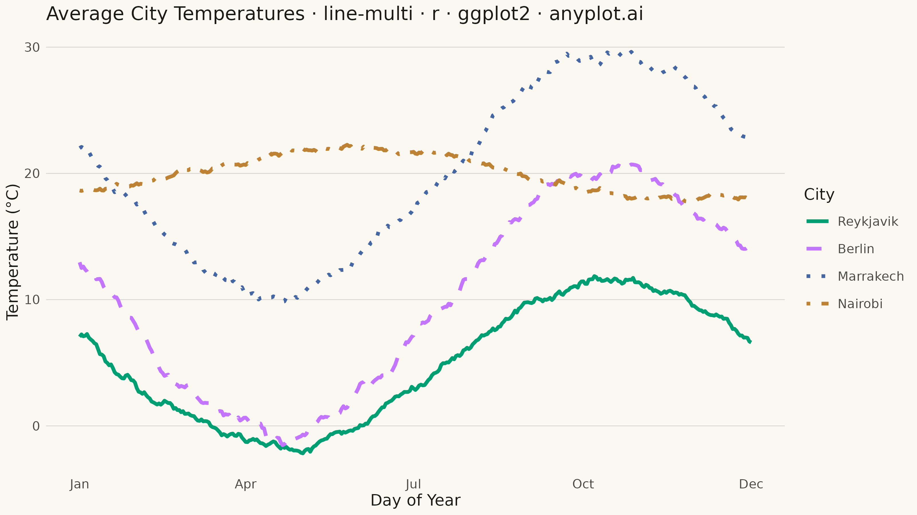
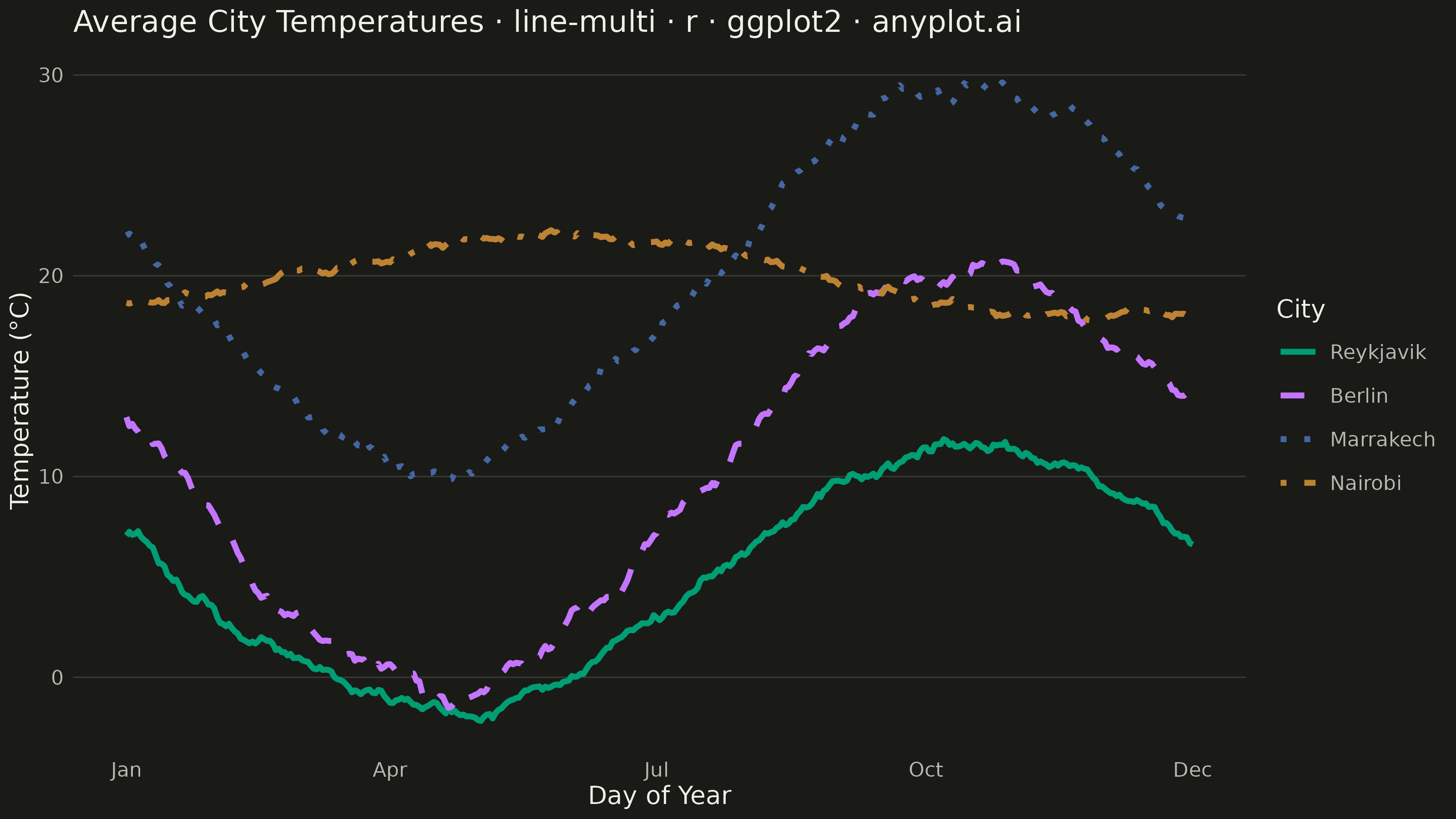
The same plot in 14 other libraries — Python: Altair, Bokeh, lets-plot, Matplotlib, Plotly, plotnine, Pygal, Seaborn; Julia: Makie.jl; JavaScript: Chart.js, D3.js, Apache ECharts, Highcharts, MUI X Charts. Compare all 15 side by side: Multi-Line Comparison Plot in Python, R, Julia and JavaScript.
A multi-line plot displays multiple data series on the same axes for direct comparison. Each series is represented by a distinct line with its own color and optional style, making it easy to identify trends, correlations, and divergences between variables. This visualization is essential for comparing related metrics over a common sequence or time period.
#' anyplot.ai
#' line-multi: Multi-Line Comparison Plot
#' Library: ggplot2 3.5.1 | R 4.4.1
#' Quality: 89/100 | Created: 2026-08-05

library(ggplot2)
library(dplyr)
library(tidyr)
library(ragg)
library(scales)

set.seed(42)

# --- Theme tokens -------------------------------------------------------
THEME    <- Sys.getenv("ANYPLOT_THEME", "light")
PAGE_BG  <- if (THEME == "light") "#FAF8F1" else "#1A1A17"
INK      <- if (THEME == "light") "#1A1A17" else "#F0EFE8"
INK_SOFT <- if (THEME == "light") "#4A4A44" else "#B8B7B0"

IMPRINT_PALETTE <- c(
  "#009E73", # 1 — brand green, always first series
  "#C475FD", # 2 — lavender
  "#4467A3", # 3 — blue
  "#BD8233"  # 4 — ochre
)

# --- Data -----------------------------------------------------------------
# Average daily temperature (°C) across a year for four cities
day_of_year <- 1:365
seasonal <- function(peak_day, amplitude, mean_temp, noise_sd) {
  mean_temp + amplitude * sin(2 * pi * (day_of_year - peak_day) / 365) +
    rnorm(length(day_of_year), 0, noise_sd)
}

temps <- tibble(
  day      = day_of_year,
  Reykjavik = seasonal(200, 6.5, 5, 1.4),
  Berlin    = seasonal(200, 10.5, 10, 1.6),
  Marrakech = seasonal(200, 9.5, 20, 1.5),
  Nairobi   = seasonal(60, 2.0, 20, 1.0)
)

df <- temps %>%
  pivot_longer(-day, names_to = "city", values_to = "temp_c") %>%
  mutate(city = factor(city, levels = c("Reykjavik", "Berlin", "Marrakech", "Nairobi")))

# Smooth each series with a rolling mean to emphasize seasonal trend over daily noise
roll_mean <- function(x, k = 7) {
  n <- length(x)
  sapply(seq_len(n), function(i) {
    lo <- max(1, i - k)
    hi <- min(n, i + k)
    mean(x[lo:hi])
  })
}

df <- df %>%
  group_by(city) %>%
  arrange(day) %>%
  mutate(temp_smooth = roll_mean(temp_c)) %>%
  ungroup()

# --- Plot -------------------------------------------------------------------
title_text <- "Average City Temperatures · line-multi · r · ggplot2 · anyplot.ai"
title_fontsize <- round(12 * min(1, 67 / nchar(title_text)))

p <- ggplot(df, aes(x = day, y = temp_smooth, color = city, linetype = city)) +
  geom_line(linewidth = 1.1) +
  scale_color_manual(values = IMPRINT_PALETTE) +
  scale_linetype_manual(values = c("solid", "dashed", "dotted", "dotdash")) +
  scale_x_continuous(
    breaks = c(1, 91, 182, 274, 365),
    labels = c("Jan", "Apr", "Jul", "Oct", "Dec")
  ) +
  labs(
    title    = title_text,
    x        = "Day of Year",
    y        = "Temperature (°C)",
    color    = "City",
    linetype = "City"
  ) +
  theme_minimal(base_size = 8) +
  theme(
    plot.background   = element_rect(fill = PAGE_BG, color = PAGE_BG),
    panel.background  = element_rect(fill = PAGE_BG, color = NA),
    panel.grid.major.x = element_blank(),
    panel.grid.minor   = element_blank(),
    panel.grid.major.y = element_line(color = scales::alpha(INK, 0.15), linewidth = 0.25),
    axis.title         = element_text(color = INK, size = 10),
    axis.text          = element_text(color = INK_SOFT, size = 8),
    axis.ticks         = element_blank(),
    plot.title         = element_text(color = INK, size = title_fontsize),
    legend.background  = element_blank(),
    legend.key         = element_blank(),
    legend.text        = element_text(color = INK_SOFT, size = 8),
    legend.title       = element_text(color = INK, size = 10),
    legend.position    = "right"
  )

# --- Save -------------------------------------------------------------------
ggsave(
  filename = sprintf("plot-%s.png", THEME),
  plot     = p,
  device   = ragg::agg_png,
  width    = 8,
  height   = 4.5,
  units    = "in",
  dpi      = 400
)
Runnable source as JSON, for any HTTP client: https://api.anyplot.ai/specs/line-multi/ggplot2/code. Any spec id and library id listed in llms-full.txt fit the same URL shape; every URL below is complete and callable.
{
  "spec_id": "line-multi",
  "language": "r",
  "library": "ggplot2",
  "page": "https://anyplot.ai/line-multi/r/ggplot2",
  "hub": "https://anyplot.ai/line-multi",
  "code_json": "https://api.anyplot.ai/specs/line-multi/ggplot2/code",
  "spec_json": "https://api.anyplot.ai/specs/line-multi",
  "render_light_png": "https://storage.googleapis.com/anyplot-images/plots/line-multi/r/ggplot2/plot-light.png",
  "render_dark_png": "https://storage.googleapis.com/anyplot-images/plots/line-multi/r/ggplot2/plot-dark.png",
  "quality_score": 89.0,
  "license": "MIT",
  "guide": "https://anyplot.ai/llms.txt"
}
Part of Multi-Line Comparison Plot on anyplot.ai.