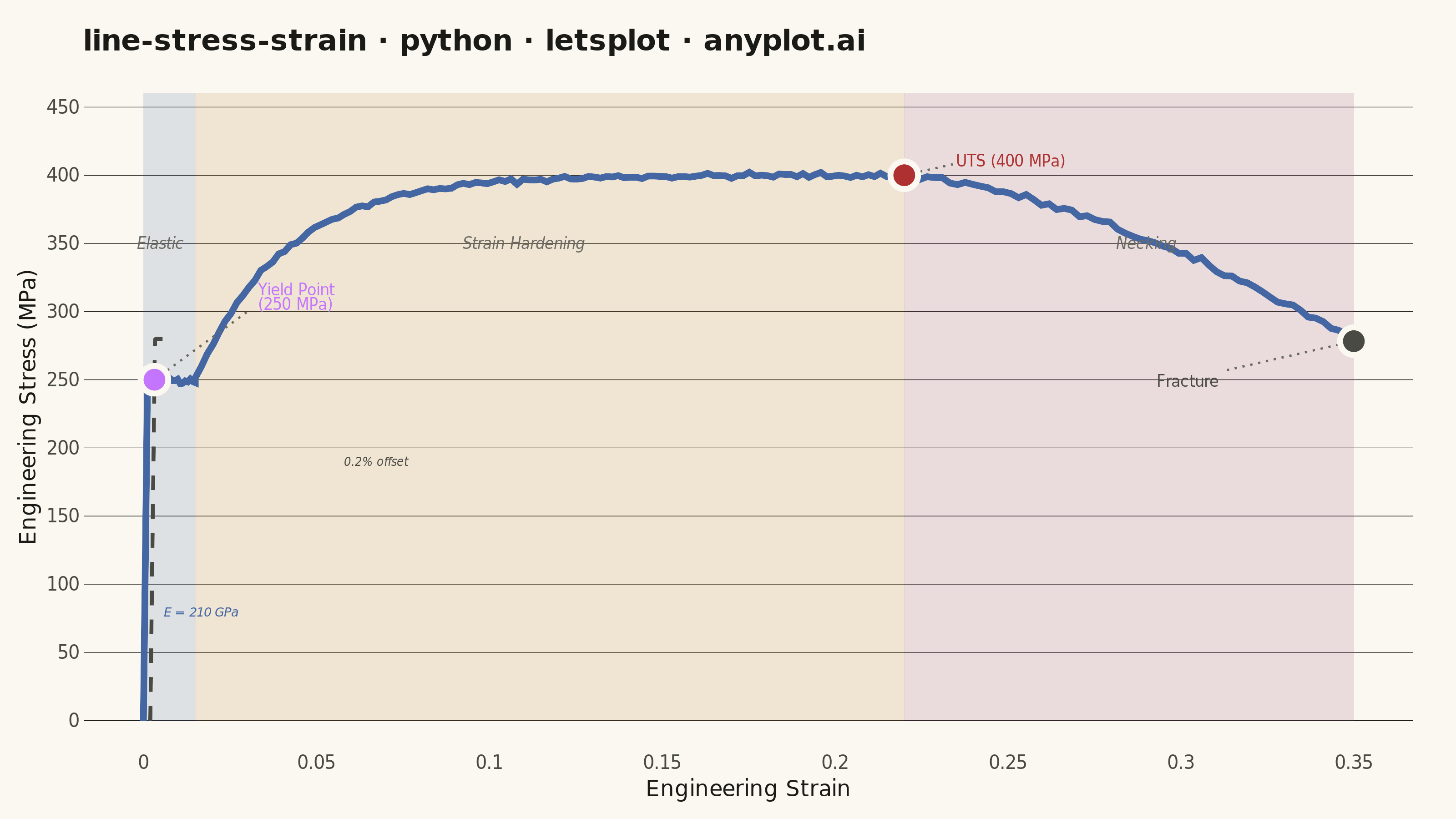
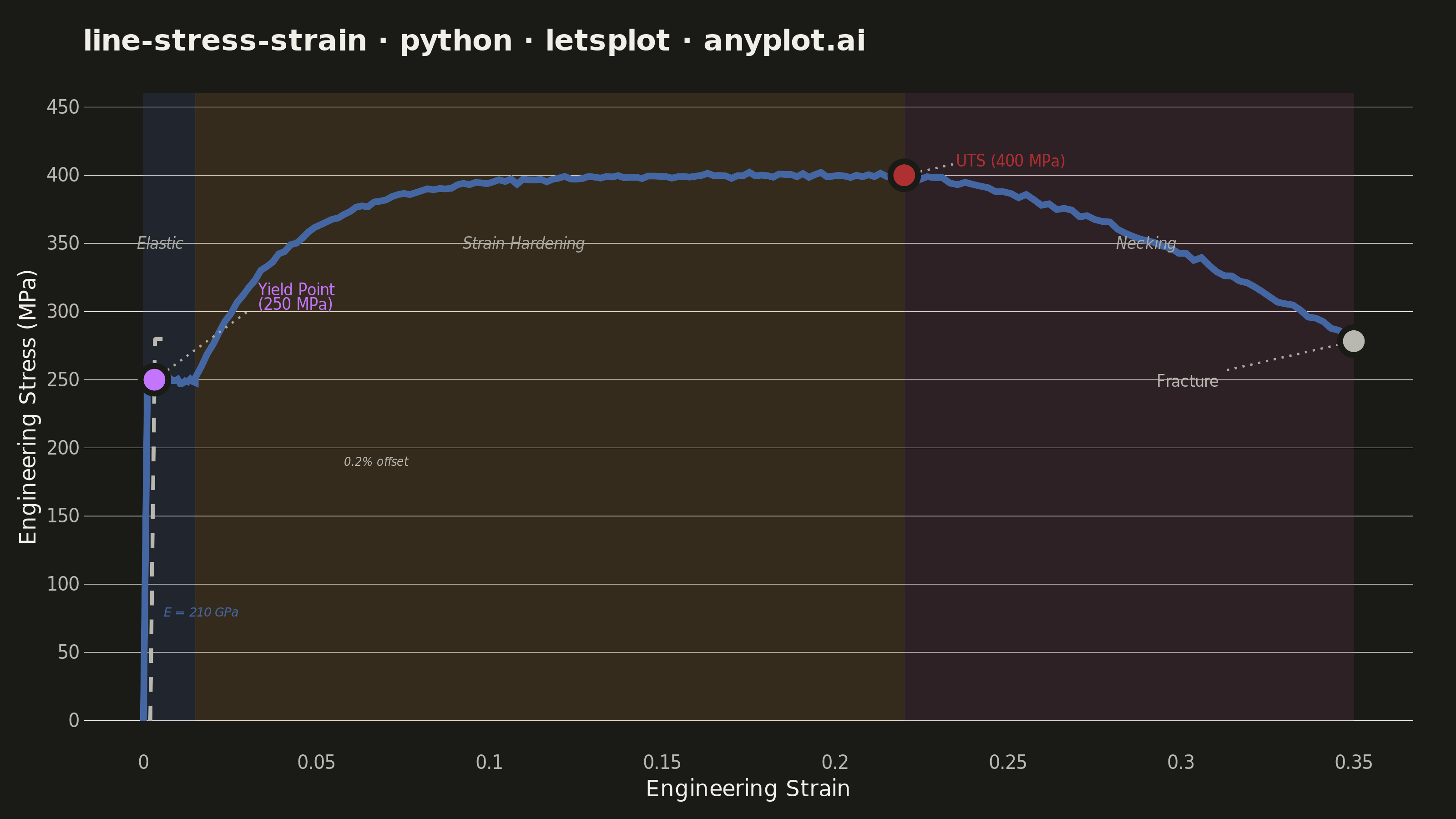
An engineering stress-strain curve visualizes the relationship between applied stress (MPa) and resulting strain (dimensionless) in a material under uniaxial tensile loading. The curve reveals distinct mechanical behavior regions — elastic deformation, yielding, strain hardening, and necking — culminating in fracture. It is the foundational plot for characterizing material mechanical properties and comparing material performance.
""" anyplot.ai
line-stress-strain: Engineering Stress-Strain Curve
Library: letsplot 4.11.0 | Python 3.13.15
Quality: 91/100 | Updated: 2026-08-17
"""

import os

import numpy as np
import pandas as pd
from lets_plot import *
from lets_plot.export import ggsave as export_ggsave


LetsPlot.setup_html()

# Theme-adaptive chrome (Imprint)
THEME = os.getenv("ANYPLOT_THEME", "light")
PAGE_BG = "#FAF8F1" if THEME == "light" else "#1A1A17"
INK = "#1A1A17" if THEME == "light" else "#F0EFE8"
INK_SOFT = "#4A4A44" if THEME == "light" else "#B8B7B0"
INK_MUTED = "#6B6A63" if THEME == "light" else "#A8A79F"

# Imprint categorical palette (theme-independent)
IMPRINT_PALETTE = ["#009E73", "#C475FD", "#4467A3", "#BD8233", "#AE3030", "#2ABCCD", "#954477", "#99B314"]

# Data - Mild steel tensile test simulation
np.random.seed(42)

# Material properties for mild steel
youngs_modulus = 210000  # MPa
yield_strength = 250  # MPa
uts = 400  # MPa (ultimate tensile strength)
fracture_strain = 0.35
uts_strain = 0.22
yield_strain = yield_strength / youngs_modulus  # ~0.00119

# Elastic region (0 to yield)
n_elastic = 60
strain_elastic = np.linspace(0, yield_strain, n_elastic)
stress_elastic = youngs_modulus * strain_elastic

# Yield plateau (mild steel has a distinct yield point)
n_plateau = 20
strain_plateau = np.linspace(yield_strain, 0.015, n_plateau)
stress_plateau = yield_strength + np.random.normal(0, 1.5, n_plateau)

# Strain hardening region (from end of plateau to UTS)
n_hardening = 120
strain_hardening = np.linspace(0.015, uts_strain, n_hardening)
stress_hardening = yield_strength + (uts - yield_strength) * (
    1 - np.exp(-8 * (strain_hardening - 0.015) / (uts_strain - 0.015))
)
stress_hardening += np.random.normal(0, 1.0, n_hardening)

# Necking region (UTS to fracture)
n_necking = 60
strain_necking = np.linspace(uts_strain, fracture_strain, n_necking)
stress_necking = uts - (uts - 280) * ((strain_necking - uts_strain) / (fracture_strain - uts_strain)) ** 1.5
stress_necking += np.random.normal(0, 1.5, n_necking)

# Combine all regions
strain = np.concatenate([strain_elastic, strain_plateau, strain_hardening, strain_necking])
stress = np.concatenate([stress_elastic, stress_plateau, stress_hardening, stress_necking])

df = pd.DataFrame({"strain": strain, "stress": stress})

# 0.2% offset line for yield point determination
offset_val = 0.002
offset_line_strain = np.linspace(offset_val, offset_val + yield_strength / youngs_modulus + 0.003, 50)
offset_line_stress = youngs_modulus * (offset_line_strain - offset_val)
offset_line_stress = np.clip(offset_line_stress, 0, yield_strength + 30)
df_offset = pd.DataFrame({"strain": offset_line_strain, "stress": offset_line_stress})

# Key points
yield_point_strain = offset_val + yield_strength / youngs_modulus
yield_point_stress = yield_strength
fracture_stress = stress_necking[-1]

df_points = pd.DataFrame(
    {
        "strain": [yield_point_strain, uts_strain, fracture_strain],
        "stress": [yield_point_stress, uts, fracture_stress],
        "type": ["Yield", "UTS", "Fracture"],
    }
)

# Consolidated annotations DataFrame (positions tuned to avoid crowding near the origin)
df_annotations = pd.DataFrame(
    {
        "x": [yield_point_strain + 0.03, uts_strain + 0.015, fracture_strain - 0.048, 0.006, 0.058, 0.005, 0.11, 0.29],
        "y": [yield_point_stress + 60, uts + 10, fracture_stress - 30, 80, 190, 350, 350, 350],
        "label": [
            f"Yield Point\n({yield_strength} MPa)",
            f"UTS ({uts} MPa)",
            "Fracture",
            f"E = {youngs_modulus // 1000} GPa",
            "0.2% offset",
            "Elastic",
            "Strain Hardening",
            "Necking",
        ],
        "group": ["yield", "uts", "fracture", "modulus", "offset", "region", "region", "region"],
    }
)

# Imprint palette roles: main curve = blue, yield = lavender, UTS = matte red (critical/peak),
# fracture = neutral ink (structural reference), 0.2% offset = neutral dashed construction line
color_main = IMPRINT_PALETTE[2]  # blue
color_yield = IMPRINT_PALETTE[1]  # lavender
color_uts = IMPRINT_PALETTE[4]  # matte red
color_fracture = INK_SOFT
color_offset = INK_SOFT

# Segment connector lines from key points to annotations (distinctive lets-plot feature)
df_segments = pd.DataFrame(
    {
        "x": [yield_point_strain, uts_strain, fracture_strain],
        "y": [yield_point_stress, uts, fracture_stress],
        "xend": [yield_point_strain + 0.028, uts_strain + 0.014, fracture_strain - 0.038],
        "yend": [yield_point_stress + 52, uts + 8, fracture_stress - 22],
    }
)

# Plot
plot = (
    ggplot()
    # Region background bands using geom_rect (distinctive lets-plot feature)
    + geom_rect(
        aes(xmin="xmin", xmax="xmax", ymin="ymin", ymax="ymax", fill="region"),
        data=pd.DataFrame(
            {
                "xmin": [0, 0.015, uts_strain],
                "xmax": [0.015, uts_strain, fracture_strain],
                "ymin": [0, 0, 0],
                "ymax": [460, 460, 460],
                "region": ["Elastic", "Strain Hardening", "Necking"],
            }
        ),
        alpha=0.16,
        color="transparent",
    )
    + scale_fill_manual(
        values={
            "Elastic": IMPRINT_PALETTE[2],
            "Strain Hardening": IMPRINT_PALETTE[3],
            "Necking": IMPRINT_PALETTE[6],
            "Yield": color_yield,
            "UTS": color_uts,
            "Fracture": color_fracture,
        }
    )
    # Main stress-strain curve with tooltips (distinctive lets-plot feature)
    + geom_line(
        aes(x="strain", y="stress"),
        data=df,
        color=color_main,
        size=1.6,
        tooltips=layer_tooltips()
        .format("strain", ".4f")
        .format("stress", ".1f")
        .line("Strain: @strain")
        .line("Stress: @stress MPa"),
    )
    # 0.2% offset line (construction reference line)
    + geom_line(aes(x="strain", y="stress"), data=df_offset, color=color_offset, size=0.9, linetype="dashed")
    # Segment connectors from points to labels (geom_segment - distinctive feature)
    + geom_segment(
        aes(x="x", y="y", xend="xend", yend="yend"), data=df_segments, color=INK_MUTED, size=0.5, linetype="dotted"
    )
    # Key points with tooltips (distinctive lets-plot feature)
    + geom_point(
        aes(x="strain", y="stress", fill="type"),
        data=df_points,
        color=PAGE_BG,
        size=5.5,
        shape=21,
        stroke=1.4,
        tooltips=layer_tooltips().line("@type").line("Strain: @strain").line("Stress: @stress MPa"),
    )
    + guides(fill="none")
    # Annotations - key points
    + geom_text(
        aes(x="x", y="y", label="label"),
        data=df_annotations.query("group == 'yield'"),
        size=4.2,
        color=color_yield,
        hjust=0,
    )
    + geom_text(
        aes(x="x", y="y", label="label"),
        data=df_annotations.query("group == 'uts'"),
        size=4.2,
        color=color_uts,
        hjust=0,
    )
    + geom_text(
        aes(x="x", y="y", label="label"),
        data=df_annotations.query("group == 'fracture'"),
        size=4.2,
        color=color_fracture,
        hjust=0.5,
    )
    # Elastic modulus annotation
    + geom_text(
        aes(x="x", y="y", label="label"),
        data=df_annotations.query("group == 'modulus'"),
        size=3.8,
        color=color_main,
        hjust=0,
        fontface="italic",
    )
    # Offset label
    + geom_text(
        aes(x="x", y="y", label="label"),
        data=df_annotations.query("group == 'offset'"),
        size=3.4,
        color=color_offset,
        hjust=0,
        fontface="italic",
    )
    # Region labels
    + geom_text(
        aes(x="x", y="y", label="label"),
        data=df_annotations.query("group == 'region'"),
        size=4.6,
        color=INK_MUTED,
        fontface="italic",
    )
    # Styling
    + labs(
        x="Engineering Strain",
        y="Engineering Stress (MPa)",
        title="line-stress-strain · python · letsplot · anyplot.ai",
    )
    + scale_x_continuous(breaks=[0, 0.05, 0.10, 0.15, 0.20, 0.25, 0.30, 0.35])
    + scale_y_continuous(breaks=[0, 50, 100, 150, 200, 250, 300, 350, 400, 450])
    + ggsize(800, 450)
    + theme_minimal()
    + theme(
        axis_text=element_text(size=10, color=INK_SOFT),
        axis_title=element_text(size=12, color=INK),
        plot_title=element_text(size=16, color=INK, face="bold"),
        panel_grid_major_x=element_blank(),
        panel_grid_major_y=element_line(color=INK, size=0.3),
        panel_grid_minor=element_blank(),
        plot_background=element_rect(fill=PAGE_BG, color=PAGE_BG),
        panel_background=element_rect(fill=PAGE_BG, color=PAGE_BG),
        panel_border=element_blank(),
        axis_ticks=element_blank(),
        axis_ticks_length=0,
        plot_margin=[15, 20, 10, 10],
    )
)

# Save
export_ggsave(plot, filename=f"plot-{THEME}.png", path=".", scale=4)
export_ggsave(plot, filename=f"plot-{THEME}.html", path=".")
Runnable source as JSON, for any HTTP client: https://api.anyplot.ai/specs/line-stress-strain/letsplot/code. Any spec id and library id listed in llms-full.txt fit the same URL shape; every URL below is complete and callable.
{
  "spec_id": "line-stress-strain",
  "language": "python",
  "library": "letsplot",
  "page": "https://anyplot.ai/line-stress-strain/python/letsplot",
  "hub": "https://anyplot.ai/line-stress-strain",
  "code_json": "https://api.anyplot.ai/specs/line-stress-strain/letsplot/code",
  "spec_json": "https://api.anyplot.ai/specs/line-stress-strain",
  "render_light_png": "https://storage.googleapis.com/anyplot-images/plots/line-stress-strain/python/letsplot/plot-light.png",
  "render_dark_png": "https://storage.googleapis.com/anyplot-images/plots/line-stress-strain/python/letsplot/plot-dark.png",
  "interactive_light_html": "https://storage.googleapis.com/anyplot-images/plots/line-stress-strain/python/letsplot/plot-light.html",
  "interactive_dark_html": "https://storage.googleapis.com/anyplot-images/plots/line-stress-strain/python/letsplot/plot-dark.html",
  "quality_score": 91.0,
  "license": "MIT",
  "guide": "https://anyplot.ai/llms.txt"
}
Part of Engineering Stress-Strain Curve on anyplot.ai.