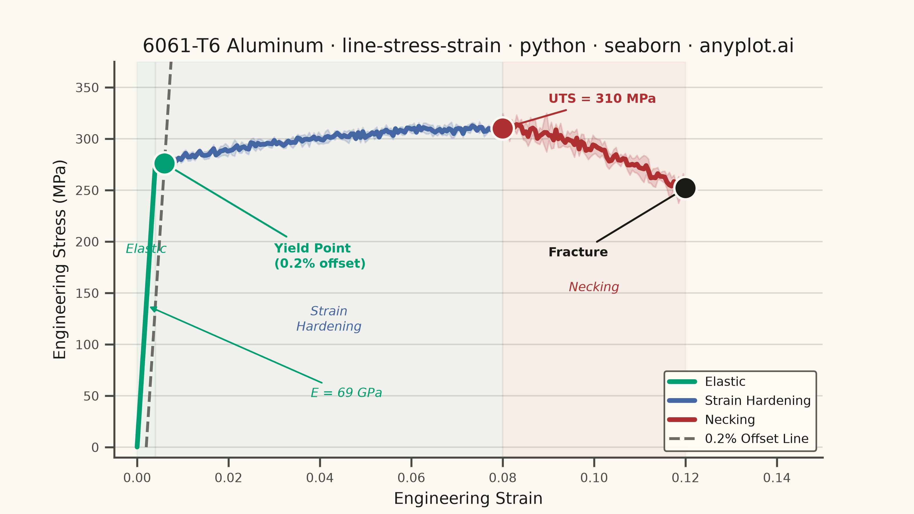
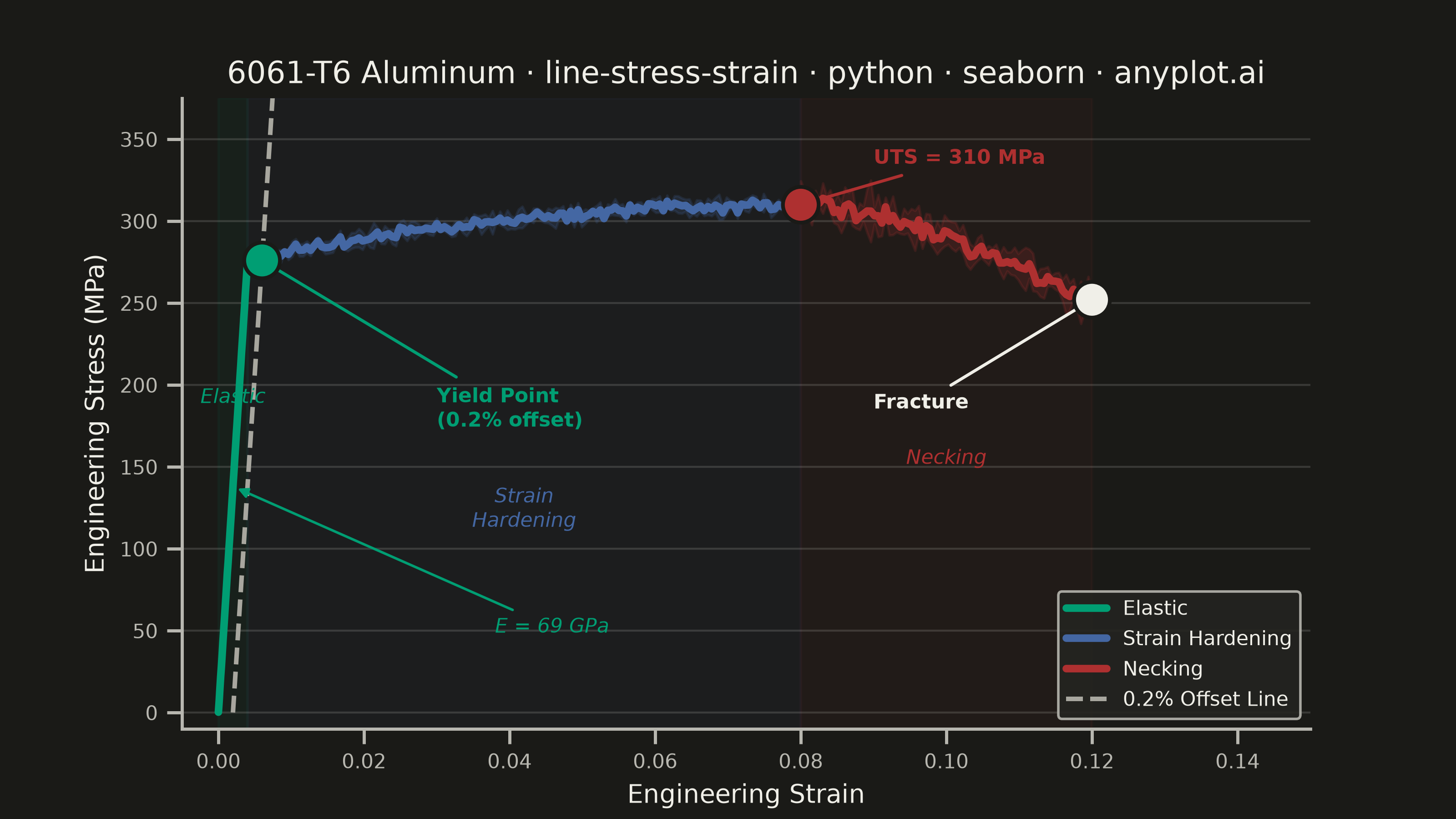
An engineering stress-strain curve visualizes the relationship between applied stress (MPa) and resulting strain (dimensionless) in a material under uniaxial tensile loading. The curve reveals distinct mechanical behavior regions — elastic deformation, yielding, strain hardening, and necking — culminating in fracture. It is the foundational plot for characterizing material mechanical properties and comparing material performance.
""" anyplot.ai
line-stress-strain: Engineering Stress-Strain Curve
Library: seaborn 0.13.2 | Python 3.13.14
Quality: 93/100 | Updated: 2026-06-21
"""

import os

import matplotlib.pyplot as plt
import numpy as np
import pandas as pd
import seaborn as sns
from matplotlib.lines import Line2D


# Theme tokens
THEME = os.getenv("ANYPLOT_THEME", "light")
PAGE_BG = "#FAF8F1" if THEME == "light" else "#1A1A17"
ELEVATED_BG = "#FFFDF6" if THEME == "light" else "#242420"
INK = "#1A1A17" if THEME == "light" else "#F0EFE8"
INK_SOFT = "#4A4A44" if THEME == "light" else "#B8B7B0"
INK_MUTED = "#6B6A63" if THEME == "light" else "#A8A79F"

# Imprint palette — canonical order, first series always #009E73
IMPRINT_PALETTE = ["#009E73", "#C475FD", "#4467A3", "#BD8233", "#AE3030", "#2ABCCD", "#954477", "#99B314"]

COLOR_ELASTIC = IMPRINT_PALETTE[0]  # brand green — first series
COLOR_HARDENING = IMPRINT_PALETTE[2]  # blue
COLOR_NECKING = IMPRINT_PALETTE[4]  # matte red — semantic: fracture/failure

# Data — Aluminum alloy 6061-T6 tensile test simulation (5 specimens)
# Different from mild steel: lower E, no yield plateau, lower ductility
np.random.seed(42)

youngs_modulus = 69_000  # MPa (69 GPa — much lower than steel's 200 GPa)
yield_stress = 276  # MPa (0.2% offset yield strength)
uts = 310  # MPa (ultimate tensile strength)
uts_strain = 0.08
fracture_strain = 0.12
fracture_stress = 252  # MPa
yield_strain = yield_stress / youngs_modulus  # ~0.004

# Shared strain grid across all specimens so seaborn can aggregate by (x, hue)
strain_elastic_ref = np.linspace(0, yield_strain, 40)
strain_hardening_ref = np.linspace(yield_strain, uts_strain, 150)
strain_necking_ref = np.linspace(uts_strain, fracture_strain, 80)

t_hard = (strain_hardening_ref - yield_strain) / (uts_strain - yield_strain)
t_neck = (strain_necking_ref - uts_strain) / (fracture_strain - uts_strain)

stress_elastic_base = youngs_modulus * strain_elastic_ref
stress_hardening_base = yield_stress + (uts - yield_stress) * (2 * t_hard - t_hard**2)
stress_necking_base = uts - (uts - fracture_stress) * t_neck**1.5

strain_all = np.concatenate([strain_elastic_ref, strain_hardening_ref, strain_necking_ref])
stress_all = np.concatenate([stress_elastic_base, stress_hardening_base, stress_necking_base])
regions = ["Elastic"] * 40 + ["Strain Hardening"] * 150 + ["Necking"] * 80

# Per-region noise scale: small in elastic (nearly deterministic linear response),
# growing through hardening, largest in necking (localised plastic instability)
noise_scale = np.concatenate(
    [
        np.full(40, 0.5),  # elastic: nearly deterministic
        np.full(150, 4.0),  # hardening: specimen-to-specimen variability
        np.full(80, 8.0),  # necking: most variable (localised deformation)
    ]
)

# Build long-format DataFrame for seaborn's statistical estimation
n_specimens = 5
specimens = []
for i in range(n_specimens):
    noise = np.random.normal(0, noise_scale)
    specimens.append(
        pd.DataFrame({"strain": strain_all, "stress": stress_all + noise, "region": regions, "specimen": i})
    )
df = pd.concat(specimens, ignore_index=True)

# 0.2% offset line (parallel to elastic slope, offset by 0.002 strain)
offset = 0.002
yield_offset_strain = offset + yield_stress / youngs_modulus  # ~0.006
yield_offset_stress = yield_stress
offset_strain = np.linspace(offset, yield_offset_strain + 0.004, 50)
offset_stress_line = youngs_modulus * (offset_strain - offset)

# Theme-adaptive chrome
sns.set_theme(
    style="ticks",
    rc={
        "figure.facecolor": PAGE_BG,
        "axes.facecolor": PAGE_BG,
        "axes.edgecolor": INK_SOFT,
        "axes.labelcolor": INK,
        "text.color": INK,
        "xtick.color": INK_SOFT,
        "ytick.color": INK_SOFT,
        "grid.color": INK,
        "grid.alpha": 0.15,
        "legend.facecolor": ELEVATED_BG,
        "legend.edgecolor": INK_SOFT,
    },
)

# Plot — canvas 3200 × 1800 px (8 in × 4.5 in @ 400 dpi)
fig, ax = plt.subplots(figsize=(8, 4.5), dpi=400)
fig.set_facecolor(PAGE_BG)
ax.set_facecolor(PAGE_BG)

region_palette = {"Elastic": COLOR_ELASTIC, "Strain Hardening": COLOR_HARDENING, "Necking": COLOR_NECKING}
region_order = ["Elastic", "Strain Hardening", "Necking"]

# Stress-strain curve coloured by region — seaborn aggregates 5 specimens,
# drawing mean line + ±1 SD band to show material-to-specimen variability
sns.lineplot(
    data=df,
    x="strain",
    y="stress",
    hue="region",
    hue_order=region_order,
    palette=region_palette,
    linewidth=3.0,
    errorbar=("sd", 1),
    err_style="band",
    err_kws={"alpha": 0.18},
    ax=ax,
    legend=False,
)

# 0.2% offset dashed line
ax.plot(offset_strain, offset_stress_line, linestyle="--", linewidth=1.8, color=INK_MUTED)

# Subtle region shading
for x0, x1, col in [
    (0, yield_strain, COLOR_ELASTIC),
    (yield_strain, uts_strain, COLOR_HARDENING),
    (uts_strain, fracture_strain, COLOR_NECKING),
]:
    ax.axvspan(x0, x1, alpha=0.05, color=col, zorder=0)

# Critical point markers (mean curve positions)
critical = pd.DataFrame(
    {
        "strain": [yield_offset_strain, uts_strain, fracture_strain],
        "stress": [yield_offset_stress, uts, fracture_stress],
        "point": ["Yield Point", "UTS", "Fracture"],
    }
)
point_palette = {"Yield Point": COLOR_ELASTIC, "UTS": COLOR_NECKING, "Fracture": INK}
sns.scatterplot(
    data=critical,
    x="strain",
    y="stress",
    hue="point",
    palette=point_palette,
    s=200,
    edgecolor=PAGE_BG,
    linewidth=1.5,
    ax=ax,
    zorder=6,
    legend=False,
)

# Annotations for key points and elastic modulus
ax.annotate(
    "Yield Point\n(0.2% offset)",
    xy=(yield_offset_strain, yield_offset_stress),
    xytext=(0.030, 200),
    fontsize=8,
    fontweight="bold",
    color=COLOR_ELASTIC,
    arrowprops={"arrowstyle": "-|>", "color": COLOR_ELASTIC, "lw": 1.2},
    ha="left",
    va="top",
)
ax.annotate(
    f"UTS = {uts} MPa",
    xy=(uts_strain, uts),
    xytext=(0.090, uts + 22),
    fontsize=8,
    fontweight="bold",
    color=COLOR_NECKING,
    arrowprops={"arrowstyle": "-|>", "color": COLOR_NECKING, "lw": 1.2},
    ha="left",
    va="bottom",
)
ax.annotate(
    "Fracture",
    xy=(fracture_strain, fracture_stress),
    xytext=(0.090, 195),
    fontsize=8,
    fontweight="bold",
    color=INK,
    arrowprops={"arrowstyle": "-|>", "color": INK, "lw": 1.2},
    ha="left",
    va="top",
)
ax.annotate(
    f"E = {youngs_modulus // 1000} GPa",
    xy=(yield_strain * 0.5, youngs_modulus * yield_strain * 0.5),
    xytext=(0.038, 52),
    fontsize=8,
    fontstyle="italic",
    color=COLOR_ELASTIC,
    arrowprops={"arrowstyle": "-|>", "color": COLOR_ELASTIC, "lw": 1.0},
    ha="left",
    va="center",
)

# Inline region labels — "Elastic" placed high in the narrow elastic zone
# (raised from 0.20 to 0.62 to reduce crowding with the E=69 GPa annotation)
ax.text(
    yield_strain / 2,
    uts * 0.62,
    "Elastic",
    fontsize=8,
    color=COLOR_ELASTIC,
    ha="center",
    va="center",
    fontstyle="italic",
)
ax.text(
    (yield_strain + uts_strain) / 2,
    uts * 0.40,
    "Strain\nHardening",
    fontsize=8,
    color=COLOR_HARDENING,
    ha="center",
    va="center",
    fontstyle="italic",
)
ax.text(
    (uts_strain + fracture_strain) / 2,
    uts * 0.50,
    "Necking",
    fontsize=8,
    color=COLOR_NECKING,
    ha="center",
    va="center",
    fontstyle="italic",
)

# Spine and grid styling
sns.despine(ax=ax)
ax.xaxis.grid(False)
ax.yaxis.grid(True, alpha=0.15, linewidth=0.8, color=INK)
ax.set_xlabel("Engineering Strain", fontsize=10, color=INK)
ax.set_ylabel("Engineering Stress (MPa)", fontsize=10, color=INK)
ax.tick_params(axis="both", labelsize=8, colors=INK_SOFT)
ax.set_xlim(-0.005, fracture_strain + 0.030)
ax.set_ylim(-10, uts + 65)

# Title with length-based font scaling (67-char baseline for seaborn = 12pt)
title = "6061-T6 Aluminum · line-stress-strain · python · seaborn · anyplot.ai"
n = len(title)
ratio = 67 / n if n > 67 else 1.0
title_fontsize = max(8, round(12 * ratio))
ax.set_title(title, fontsize=title_fontsize, fontweight="medium", color=INK)

# Manual legend (three regions + offset line)
legend_handles = [
    Line2D([0], [0], color=COLOR_ELASTIC, linewidth=3.0, label="Elastic"),
    Line2D([0], [0], color=COLOR_HARDENING, linewidth=3.0, label="Strain Hardening"),
    Line2D([0], [0], color=COLOR_NECKING, linewidth=3.0, label="Necking"),
    Line2D([0], [0], color=INK_MUTED, linewidth=1.8, linestyle="--", label="0.2% Offset Line"),
]
ax.legend(
    handles=legend_handles, fontsize=8, loc="lower right", framealpha=0.9, facecolor=ELEVATED_BG, edgecolor=INK_SOFT
)

# Save — no bbox_inches to preserve exact 3200×1800 canvas
plt.savefig(f"plot-{THEME}.png", dpi=400, facecolor=PAGE_BG)
plt.close()
Runnable source as JSON, for any HTTP client: https://api.anyplot.ai/specs/line-stress-strain/seaborn/code. Any spec id and library id listed in llms-full.txt fit the same URL shape; every URL below is complete and callable.
{
  "spec_id": "line-stress-strain",
  "language": "python",
  "library": "seaborn",
  "page": "https://anyplot.ai/line-stress-strain/python/seaborn",
  "hub": "https://anyplot.ai/line-stress-strain",
  "code_json": "https://api.anyplot.ai/specs/line-stress-strain/seaborn/code",
  "spec_json": "https://api.anyplot.ai/specs/line-stress-strain",
  "render_light_png": "https://storage.googleapis.com/anyplot-images/plots/line-stress-strain/python/seaborn/plot-light.png",
  "render_dark_png": "https://storage.googleapis.com/anyplot-images/plots/line-stress-strain/python/seaborn/plot-dark.png",
  "quality_score": 93.0,
  "license": "MIT",
  "guide": "https://anyplot.ai/llms.txt"
}
Part of Engineering Stress-Strain Curve on anyplot.ai.