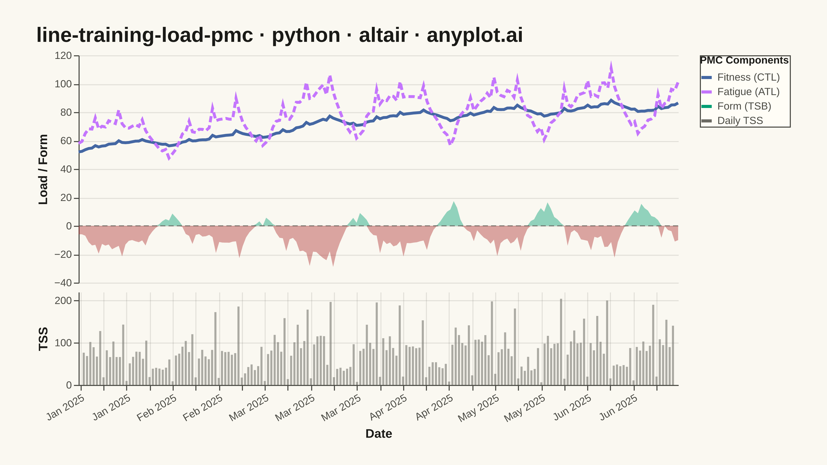
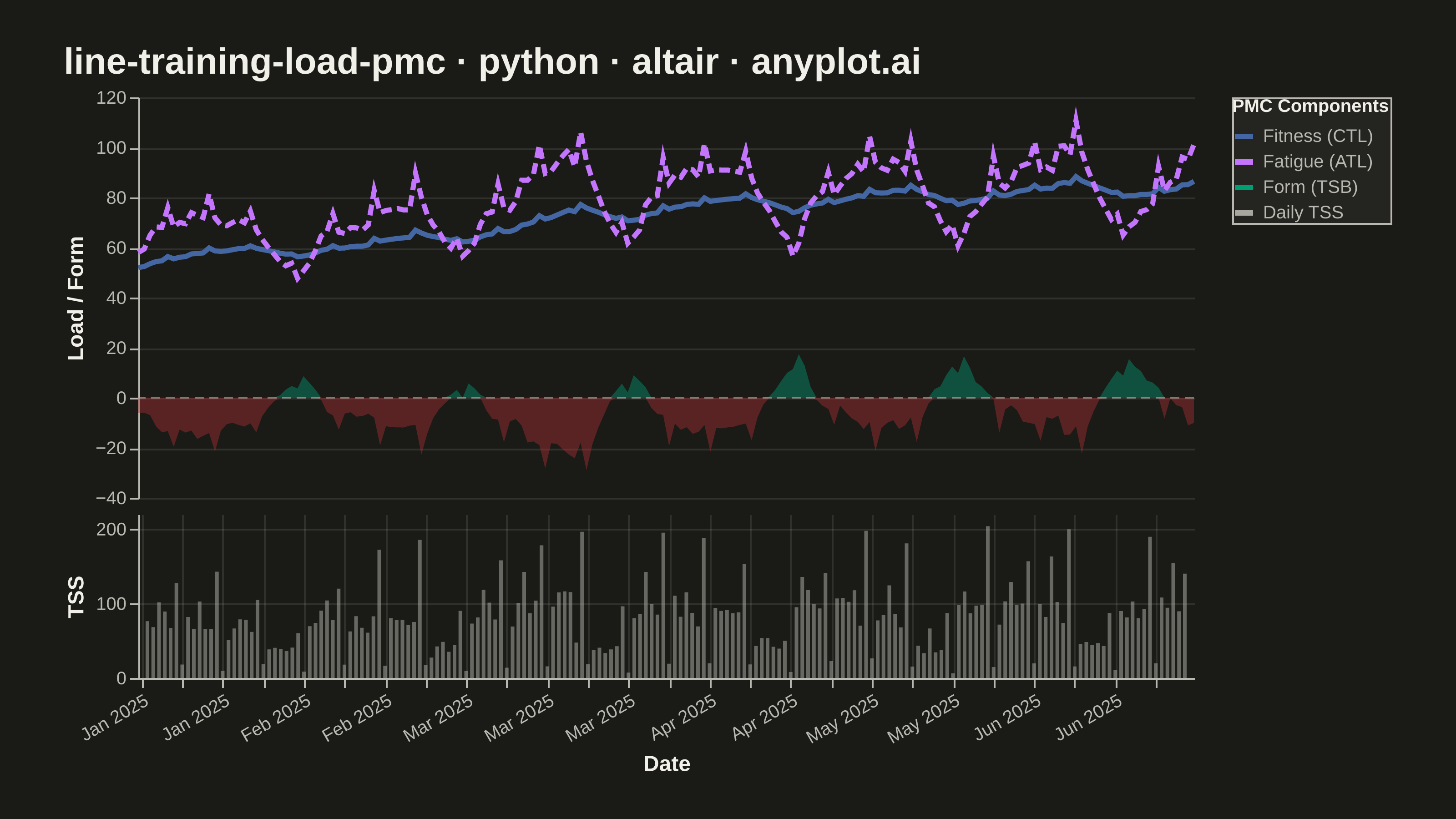
A Performance Management Chart (PMC), popularized by TrainingPeaks, summarizes an endurance athlete's training history on a single shared time axis. Two exponentially-smoothed lines track Chronic Training Load (CTL, "fitness", ~42-day time constant) and Acute Training Load (ATL, "fatigue", ~7-day time constant), while a filled area or band shows Training Stress Balance (TSB, "form" = CTL − ATL) above and below a zero baseline. Daily Training Stress Score (TSS) values appear as points or thin vertical bars, giving the raw workout intensity behind the smoothed trends. The chart reveals whether an athlete is building fitness, accumulating fatigue, or freshening up (positive form) for a target event.
""" anyplot.ai
line-training-load-pmc: Training Load Performance Management Chart
Library: altair 6.2.1 | Python 3.13.13
Quality: 87/100 | Created: 2026-06-13
"""

import os
import sys


# Remove script directory from sys.path to avoid importing local altair.py
_script_dir = os.path.dirname(os.path.abspath(__file__))
if _script_dir in sys.path:
    sys.path.remove(_script_dir)
sys.path[:] = [p for p in sys.path if os.path.abspath(p or ".") != _script_dir]

import altair as alt
import numpy as np
import pandas as pd
from PIL import Image


# Theme tokens
THEME = os.getenv("ANYPLOT_THEME", "light")
PAGE_BG = "#FAF8F1" if THEME == "light" else "#1A1A17"
ELEVATED_BG = "#FFFDF6" if THEME == "light" else "#242420"
INK = "#1A1A17" if THEME == "light" else "#F0EFE8"
INK_SOFT = "#4A4A44" if THEME == "light" else "#B8B7B0"
INK_MUTED = "#6B6A63" if THEME == "light" else "#A8A79F"

# Imprint palette — semantic assignment for PMC metrics
COLOR_CTL = "#4467A3"  # blue — fitness/chronic (smooth, rising)
COLOR_ATL = "#C475FD"  # lavender — fatigue/acute (volatile)
COLOR_TSB_POS = "#009E73"  # brand green — positive form (fresh)
COLOR_TSB_NEG = "#AE3030"  # matte red — negative form (fatigued)
COLOR_TSS = INK_MUTED  # muted neutral — raw daily load bars

# Data — 180-day training block with realistic PMC values
np.random.seed(42)
n_days = 180
dates = pd.date_range("2025-01-06", periods=n_days, freq="D")

# Simulate TSS: weekly structure, 3-week build + 1-week recovery mesocycle
tss_raw = np.zeros(n_days)
for i in range(n_days):
    week = i // 7
    day_of_week = i % 7
    recovery_week = week % 4 == 3
    base = 40 if recovery_week else 70 + min(week, 12) * 2.0
    if day_of_week == 5:  # Saturday long workout
        base *= 1.9
    elif day_of_week == 6:  # Sunday easy/rest
        base *= 0.2
    elif day_of_week == 2:  # Wednesday quality session
        base *= 1.3
    tss_raw[i] = max(0.0, np.random.normal(base, base * 0.18))

# PMC EWMA — seed CTL/ATL realistically (trained athlete starting value)
ctl = np.zeros(n_days)
atl = np.zeros(n_days)
tsb = np.zeros(n_days)
alpha_ctl = 1 - np.exp(-1 / 42)
alpha_atl = 1 - np.exp(-1 / 7)

ctl[0] = 52.0  # realistic fitness base at start of block
atl[0] = 58.0  # slightly elevated fatigue at block start
tsb[0] = ctl[0] - atl[0]

for i in range(1, n_days):
    ctl[i] = ctl[i - 1] + alpha_ctl * (tss_raw[i] - ctl[i - 1])
    atl[i] = atl[i - 1] + alpha_atl * (tss_raw[i] - atl[i - 1])
    tsb[i] = ctl[i - 1] - atl[i - 1]  # previous-day values per PMC convention

df_main = pd.DataFrame({"date": dates, "ctl": ctl, "atl": atl, "tsb": tsb})
df_tss = pd.DataFrame({"date": dates, "tss": tss_raw})
df_tsb_pos = df_main[["date"]].copy()
df_tsb_pos["tsb_pos"] = df_main["tsb"].clip(lower=0)
df_tsb_neg = df_main[["date"]].copy()
df_tsb_neg["tsb_neg"] = df_main["tsb"].clip(upper=0)

# Title sizing
title_str = "line-training-load-pmc · python · altair · anyplot.ai"
n_chars = len(title_str)
title_fontsize = max(round(16 * 67 / n_chars), 11)

# ── Top panel: CTL / ATL lines + TSB filled areas (shared y-axis) ────────────
# Shared y spans CTL/ATL range (~30-100) and TSB range (~-40 to +30) together.
# TSB fills use y/y2 anchored at 0; all layers share one axis → no label clash.

tsb_pos_area = (
    alt.Chart(df_tsb_pos)
    .mark_area(color=COLOR_TSB_POS, opacity=0.42, line=False)
    .encode(x=alt.X("date:T", axis=None), y=alt.Y("tsb_pos:Q", title="Load / Form"), y2=alt.Y2(datum=0))
)
tsb_neg_area = (
    alt.Chart(df_tsb_neg)
    .mark_area(color=COLOR_TSB_NEG, opacity=0.42, line=False)
    .encode(x=alt.X("date:T", axis=None), y=alt.Y("tsb_neg:Q"), y2=alt.Y2(datum=0))
)
tsb_zero = (
    alt.Chart(pd.DataFrame({"y": [0]}))
    .mark_rule(color=INK_SOFT, strokeWidth=1, strokeDash=[5, 3], opacity=0.6)
    .encode(y=alt.Y("y:Q"))
)

# Melt CTL/ATL into long form for a clean colour-encoded legend
df_lines = df_main[["date", "ctl", "atl"]].melt(id_vars="date", var_name="metric", value_name="value")
df_lines["metric"] = df_lines["metric"].map({"ctl": "Fitness (CTL)", "atl": "Fatigue (ATL)"})

# Add dummy entries so TSB and TSS appear in the shared legend (NaN = no visible line rendered)
df_legend_extras = pd.DataFrame(
    {"date": [dates[0], dates[0]], "metric": ["Form (TSB)", "Daily TSS"], "value": [np.nan, np.nan]}
)
df_lines = pd.concat([df_lines, df_legend_extras], ignore_index=True)

_LEGEND_DOMAIN = ["Fitness (CTL)", "Fatigue (ATL)", "Form (TSB)", "Daily TSS"]
_LEGEND_COLORS = [COLOR_CTL, COLOR_ATL, COLOR_TSB_POS, COLOR_TSS]

metric_lines = (
    alt.Chart(df_lines)
    .mark_line(strokeWidth=2.8)
    .encode(
        x=alt.X("date:T", axis=None),
        y=alt.Y(
            "value:Q",
            title="Load / Form",
            axis=alt.Axis(labelFontSize=10, titleFontSize=12, titleColor=INK, labelColor=INK_SOFT),
        ),
        color=alt.Color(
            "metric:N",
            scale=alt.Scale(domain=_LEGEND_DOMAIN, range=_LEGEND_COLORS),
            legend=alt.Legend(
                title="PMC Components", orient="right", symbolStrokeWidth=3, labelFontSize=10, titleFontSize=10
            ),
        ),
        strokeDash=alt.condition(alt.datum.metric == "Fatigue (ATL)", alt.value([6, 3]), alt.value([1, 0])),
        tooltip=[
            alt.Tooltip("date:T", format="%b %d"),
            alt.Tooltip("metric:N", title="Series"),
            alt.Tooltip("value:Q", format=".1f"),
        ],
    )
)

top_panel = alt.layer(tsb_pos_area, tsb_neg_area, tsb_zero, metric_lines).properties(width=580, height=220)

# ── Bottom panel: daily TSS bars ─────────────────────────────────────────────
tss_bars = (
    alt.Chart(df_tss)
    .mark_bar(color=COLOR_TSS, opacity=0.55, width=2)
    .encode(
        x=alt.X(
            "date:T",
            title="Date",
            axis=alt.Axis(
                format="%b %Y", labelAngle=-30, labelFontSize=10, titleFontSize=12, titleColor=INK, labelColor=INK_SOFT
            ),
        ),
        y=alt.Y(
            "tss:Q", title="TSS", axis=alt.Axis(labelFontSize=10, titleFontSize=12, titleColor=INK, labelColor=INK_SOFT)
        ),
        tooltip=[alt.Tooltip("date:T", format="%b %d"), alt.Tooltip("tss:Q", title="TSS", format=".0f")],
    )
    .properties(width=580, height=90)
)

# ── Compose full chart ────────────────────────────────────────────────────────
chart = (
    alt.vconcat(top_panel, tss_bars, spacing=4)
    .properties(
        background=PAGE_BG, title=alt.TitleParams(text=title_str, fontSize=title_fontsize, color=INK, anchor="start")
    )
    .configure_view(fill=PAGE_BG, stroke=None)
    .configure_axis(
        domainColor=INK_SOFT, tickColor=INK_SOFT, gridColor=INK, gridOpacity=0.10, labelColor=INK_SOFT, titleColor=INK
    )
    .configure_legend(
        fillColor=ELEVATED_BG,
        strokeColor=INK_SOFT,
        labelColor=INK_SOFT,
        titleColor=INK,
        labelFontSize=10,
        titleFontSize=10,
    )
)

# Save PNG then pad to exact 3200×1800
chart.save(f"plot-{THEME}.png", scale_factor=4.0)

TW, TH = 3200, 1800
_img = Image.open(f"plot-{THEME}.png").convert("RGB")
_w, _h = _img.size
if _w > TW or _h > TH:
    raise SystemExit(
        f"altair vl-convert produced {_w}×{_h}, exceeds target {TW}×{TH}. "
        f"Shrink chart .properties(width=, height=) values and re-render."
    )
if _w < TW or _h < TH:
    _canvas = Image.new("RGB", (TW, TH), PAGE_BG)
    _canvas.paste(_img, ((TW - _w) // 2, (TH - _h) // 2))
    _canvas.save(f"plot-{THEME}.png")

# Save interactive HTML
chart.save(f"plot-{THEME}.html")
Runnable source as JSON, for any HTTP client: https://api.anyplot.ai/specs/line-training-load-pmc/altair/code. Any spec id and library id listed in llms-full.txt fit the same URL shape; every URL below is complete and callable.
{
  "spec_id": "line-training-load-pmc",
  "language": "python",
  "library": "altair",
  "page": "https://anyplot.ai/line-training-load-pmc/python/altair",
  "hub": "https://anyplot.ai/line-training-load-pmc",
  "code_json": "https://api.anyplot.ai/specs/line-training-load-pmc/altair/code",
  "spec_json": "https://api.anyplot.ai/specs/line-training-load-pmc",
  "render_light_png": "https://storage.googleapis.com/anyplot-images/plots/line-training-load-pmc/python/altair/plot-light.png",
  "render_dark_png": "https://storage.googleapis.com/anyplot-images/plots/line-training-load-pmc/python/altair/plot-dark.png",
  "interactive_light_html": "https://storage.googleapis.com/anyplot-images/plots/line-training-load-pmc/python/altair/plot-light.html",
  "interactive_dark_html": "https://storage.googleapis.com/anyplot-images/plots/line-training-load-pmc/python/altair/plot-dark.html",
  "quality_score": 87.0,
  "license": "MIT",
  "guide": "https://anyplot.ai/llms.txt"
}
Part of Training Load Performance Management Chart on anyplot.ai.