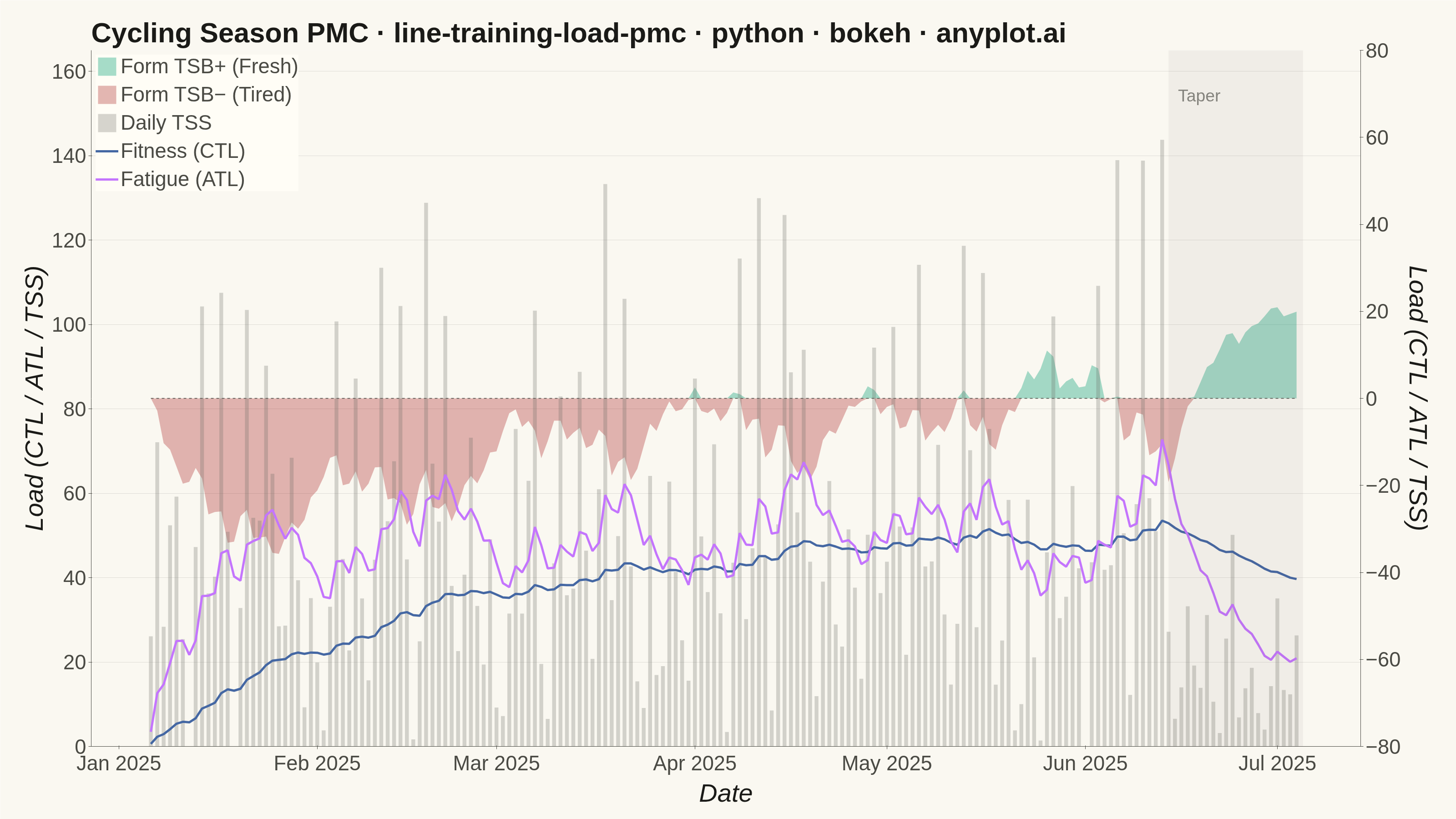
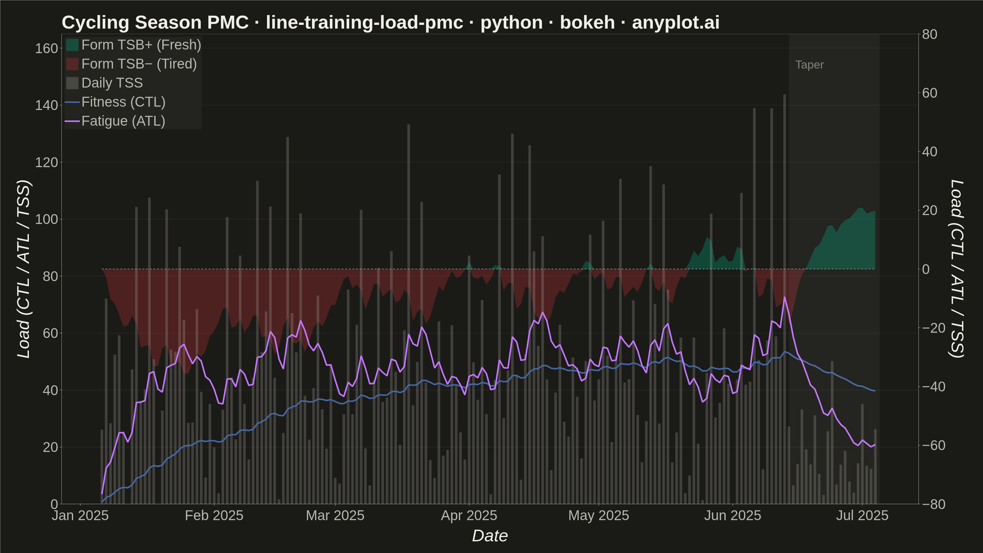
A Performance Management Chart (PMC), popularized by TrainingPeaks, summarizes an endurance athlete's training history on a single shared time axis. Two exponentially-smoothed lines track Chronic Training Load (CTL, "fitness", ~42-day time constant) and Acute Training Load (ATL, "fatigue", ~7-day time constant), while a filled area or band shows Training Stress Balance (TSB, "form" = CTL − ATL) above and below a zero baseline. Daily Training Stress Score (TSS) values appear as points or thin vertical bars, giving the raw workout intensity behind the smoothed trends. The chart reveals whether an athlete is building fitness, accumulating fatigue, or freshening up (positive form) for a target event.
""" anyplot.ai
line-training-load-pmc: Training Load Performance Management Chart
Library: bokeh 3.9.1 | Python 3.13.13
Quality: 90/100 | Created: 2026-06-13
"""

import os
import sys


# Prevent self-import: this file is named bokeh.py, which shadows the installed
# bokeh package when its directory sits at the front of sys.path.
_this_dir = os.path.dirname(os.path.abspath(__file__))
sys.path = [p for p in sys.path if os.path.abspath(p or ".") != _this_dir]

import time
from pathlib import Path

import numpy as np
import pandas as pd
from bokeh.io import output_file, save
from bokeh.models import BoxAnnotation, ColumnDataSource, Label, LinearAxis, Range1d
from bokeh.plotting import figure
from selenium import webdriver
from selenium.webdriver.chrome.options import Options


# Theme tokens
THEME = os.getenv("ANYPLOT_THEME", "light")
PAGE_BG = "#FAF8F1" if THEME == "light" else "#1A1A17"
ELEVATED_BG = "#FFFDF6" if THEME == "light" else "#242420"
INK = "#1A1A17" if THEME == "light" else "#F0EFE8"
INK_SOFT = "#4A4A44" if THEME == "light" else "#B8B7B0"
INK_MUTED = "#6B6A63" if THEME == "light" else "#A8A79F"

# Imprint palette — semantic mapping for PMC chart
TSB_FRESH = "#009E73"  # brand green — positive form (fresh)
CTL_COLOR = "#4467A3"  # blue — fitness / chronic load
ATL_COLOR = "#C475FD"  # lavender — fatigue / acute load
TSB_TIRED = "#AE3030"  # matte red — negative form (fatigued)

# Data: 180-day cycling training block
np.random.seed(42)
n_days = 180
dates = pd.date_range(start="2025-01-06", periods=n_days, freq="D")

# Generate realistic TSS: 3-week build + 1-week recovery cycles, taper at end
tss = np.zeros(n_days)
for i in range(n_days):
    week = i // 7
    day_in_week = i % 7
    week_in_block = week % 4
    load_factor = [0.70, 0.85, 1.00, 0.45][week_in_block]

    if day_in_week == 6:
        base = np.random.uniform(0, 20)
    elif day_in_week in [1, 4]:
        base = np.random.uniform(90, 150) * load_factor
    else:
        base = np.random.uniform(35, 75) * load_factor

    tss[i] = max(0, base + np.random.normal(0, 8))

# Three-week taper before target race
tss[n_days - 21 : n_days - 10] *= 0.55
tss[n_days - 10 :] *= 0.25

# CTL (42-day EWMA) and ATL (7-day EWMA)
ctl_alpha = 1 - np.exp(-1 / 42)
atl_alpha = 1 - np.exp(-1 / 7)

ctl = np.zeros(n_days)
atl = np.zeros(n_days)
ctl[0] = tss[0] * ctl_alpha
atl[0] = tss[0] * atl_alpha

for i in range(1, n_days):
    ctl[i] = (1 - ctl_alpha) * ctl[i - 1] + ctl_alpha * tss[i]
    atl[i] = (1 - atl_alpha) * atl[i - 1] + atl_alpha * tss[i]

# TSB = previous-day CTL minus previous-day ATL
tsb = np.zeros(n_days)
for i in range(1, n_days):
    tsb[i] = ctl[i - 1] - atl[i - 1]

# Split TSB for two-toned fill
tsb_pos = np.where(tsb >= 0, tsb, 0.0)
tsb_neg = np.where(tsb < 0, tsb, 0.0)
zeros = np.zeros(n_days)

# Title — length-scaled font (baseline 50pt for ~67 chars)
title = "Cycling Season PMC · line-training-load-pmc · python · bokeh · anyplot.ai"
n = len(title)
ratio = 67 / n if n > 67 else 1.0
title_size = f"{max(34, round(50 * ratio))}pt"

# Figure: primary y for CTL/ATL/TSS, secondary y for TSB
p = figure(
    width=3200,
    height=1800,
    x_axis_type="datetime",
    y_range=Range1d(start=0, end=165),
    toolbar_location=None,
    min_border_bottom=160,
    min_border_left=200,
    min_border_top=110,
    min_border_right=210,
)

# Secondary y-axis for TSB (right side)
p.extra_y_ranges = {"tsb": Range1d(start=-80, end=80)}
tsb_axis = LinearAxis(
    y_range_name="tsb",
    axis_label="Form (TSB)",
    axis_label_text_font_size="42pt",
    axis_label_text_color=INK,
    major_label_text_font_size="34pt",
    major_label_text_color=INK_SOFT,
    axis_line_color=None,
    major_tick_line_color=INK_SOFT,
    minor_tick_line_color=None,
)
p.add_layout(tsb_axis, "right")

# ColumnDataSource
source = ColumnDataSource(
    data={"dates": dates, "tss": tss, "ctl": ctl, "atl": atl, "tsb_pos": tsb_pos, "tsb_neg": tsb_neg, "zeros": zeros}
)

# Draw order: TSB areas → zero reference → TSS bars → CTL line → ATL line
# TSB positive area (fresh / green) — first series, always Imprint position 1
p.varea(
    x="dates",
    y1="zeros",
    y2="tsb_pos",
    source=source,
    y_range_name="tsb",
    fill_color=TSB_FRESH,
    fill_alpha=0.35,
    legend_label="Form TSB+ (Fresh)",
)

# TSB negative area (fatigued / red)
p.varea(
    x="dates",
    y1="tsb_neg",
    y2="zeros",
    source=source,
    y_range_name="tsb",
    fill_color=TSB_TIRED,
    fill_alpha=0.35,
    legend_label="Form TSB− (Tired)",
)

# TSB = 0 reference line (no legend entry — structural chrome)
p.line(x="dates", y="zeros", source=source, y_range_name="tsb", line_color=INK_SOFT, line_width=1.5, line_dash="dashed")

# Daily TSS bars — subordinate raw input
day_ms = 86_400_000
p.vbar(
    x="dates",
    top="tss",
    bottom=0,
    width=day_ms * 0.60,
    source=source,
    fill_color=INK_MUTED,
    fill_alpha=0.28,
    line_color=None,
    legend_label="Daily TSS",
)

# CTL line — fitness / chronic load
p.line(x="dates", y="ctl", source=source, line_color=CTL_COLOR, line_width=5.0, legend_label="Fitness (CTL)")

# ATL line — fatigue / acute load
p.line(x="dates", y="atl", source=source, line_color=ATL_COLOR, line_width=5.0, legend_label="Fatigue (ATL)")

# Taper region annotation — final 21 days where load was progressively reduced
# Draws attention to the race-preparation narrative (DE-03 storytelling)
taper_start_ms = float(dates[n_days - 21].value) / 1_000_000  # ns → ms (bokeh datetime axis unit)
taper_end_ms = float(dates[-1].value) / 1_000_000 + 86_400_000  # include last day
taper_box = BoxAnnotation(
    left=taper_start_ms, right=taper_end_ms, fill_color=INK_MUTED, fill_alpha=0.07, line_color=None
)
p.add_layout(taper_box)
taper_label = Label(
    x=taper_start_ms,
    y=152,
    text="  Taper",
    text_color=INK_SOFT,
    text_font_size="28pt",
    text_alpha=0.65,
    x_units="data",
    y_units="data",
)
p.add_layout(taper_label)

# Theme chrome
p.background_fill_color = PAGE_BG
p.border_fill_color = PAGE_BG
p.outline_line_color = None

p.title.text = title
p.title.text_font_size = title_size
p.title.text_color = INK
p.title.text_font_style = "bold"

p.xaxis.axis_label = "Date"
p.xaxis.axis_label_text_font_size = "42pt"
p.xaxis.axis_label_text_color = INK
p.xaxis.major_label_text_font_size = "34pt"
p.xaxis.major_label_text_color = INK_SOFT
p.xaxis.axis_line_color = INK_SOFT
p.xaxis.major_tick_line_color = INK_SOFT
p.xaxis.minor_tick_line_color = None

p.yaxis.axis_label = "Load (CTL / ATL / TSS)"
p.yaxis.axis_label_text_font_size = "42pt"
p.yaxis.axis_label_text_color = INK
p.yaxis.major_label_text_font_size = "34pt"
p.yaxis.major_label_text_color = INK_SOFT
p.yaxis.axis_line_color = INK_SOFT
p.yaxis.major_tick_line_color = INK_SOFT
p.yaxis.minor_tick_line_color = None

p.xgrid.grid_line_color = None
p.ygrid.grid_line_color = INK
p.ygrid.grid_line_alpha = 0.12

# Legend
p.legend.location = "top_left"
p.legend.background_fill_color = ELEVATED_BG
p.legend.border_line_color = None
p.legend.label_text_color = INK_SOFT
p.legend.label_text_font_size = "34pt"
p.legend.glyph_width = 50
p.legend.glyph_height = 50
p.legend.spacing = 10
p.legend.padding = 16
p.legend.click_policy = "hide"

# Save HTML (interactive catalog artifact)
output_file(f"plot-{THEME}.html")
save(p)

# Screenshot with headless Selenium (Bokeh export_png not available in CI)
W, H = 3200, 1800
opts = Options()
for arg in (
    "--headless=new",
    "--no-sandbox",
    "--disable-dev-shm-usage",
    "--disable-gpu",
    f"--window-size={W},{H}",
    "--hide-scrollbars",
):
    opts.add_argument(arg)
driver = webdriver.Chrome(options=opts)
# CDP override forces an exact W×H viewport regardless of outer window chrome
driver.execute_cdp_cmd(
    "Emulation.setDeviceMetricsOverride", {"width": W, "height": H, "deviceScaleFactor": 1, "mobile": False}
)
driver.get(f"file://{Path(f'plot-{THEME}.html').resolve()}")
time.sleep(3)
driver.save_screenshot(f"plot-{THEME}.png")
driver.quit()
Runnable source as JSON, for any HTTP client: https://api.anyplot.ai/specs/line-training-load-pmc/bokeh/code. Any spec id and library id listed in llms-full.txt fit the same URL shape; every URL below is complete and callable.
{
  "spec_id": "line-training-load-pmc",
  "language": "python",
  "library": "bokeh",
  "page": "https://anyplot.ai/line-training-load-pmc/python/bokeh",
  "hub": "https://anyplot.ai/line-training-load-pmc",
  "code_json": "https://api.anyplot.ai/specs/line-training-load-pmc/bokeh/code",
  "spec_json": "https://api.anyplot.ai/specs/line-training-load-pmc",
  "render_light_png": "https://storage.googleapis.com/anyplot-images/plots/line-training-load-pmc/python/bokeh/plot-light.png",
  "render_dark_png": "https://storage.googleapis.com/anyplot-images/plots/line-training-load-pmc/python/bokeh/plot-dark.png",
  "interactive_light_html": "https://storage.googleapis.com/anyplot-images/plots/line-training-load-pmc/python/bokeh/plot-light.html",
  "interactive_dark_html": "https://storage.googleapis.com/anyplot-images/plots/line-training-load-pmc/python/bokeh/plot-dark.html",
  "quality_score": 90.0,
  "license": "MIT",
  "guide": "https://anyplot.ai/llms.txt"
}
Part of Training Load Performance Management Chart on anyplot.ai.