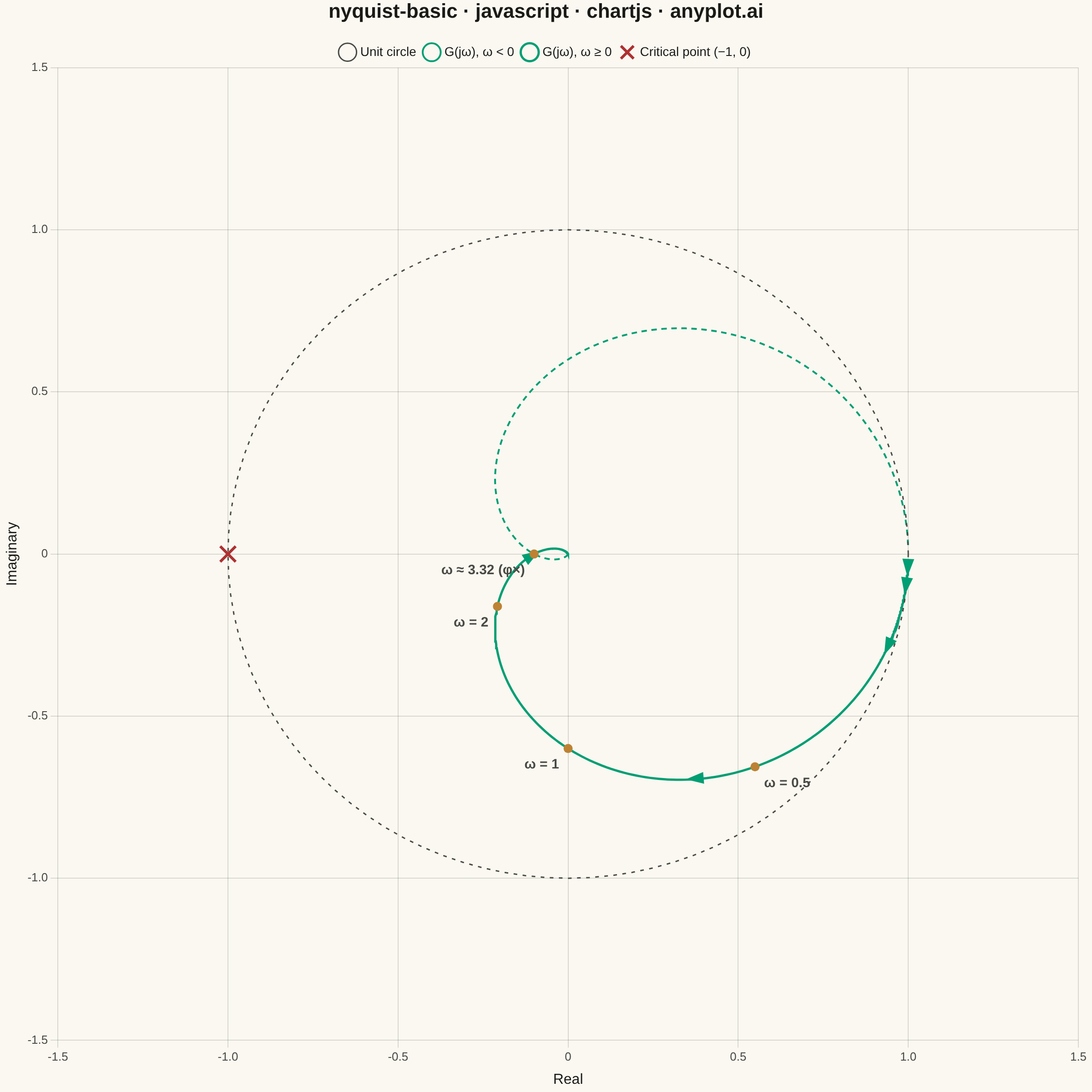
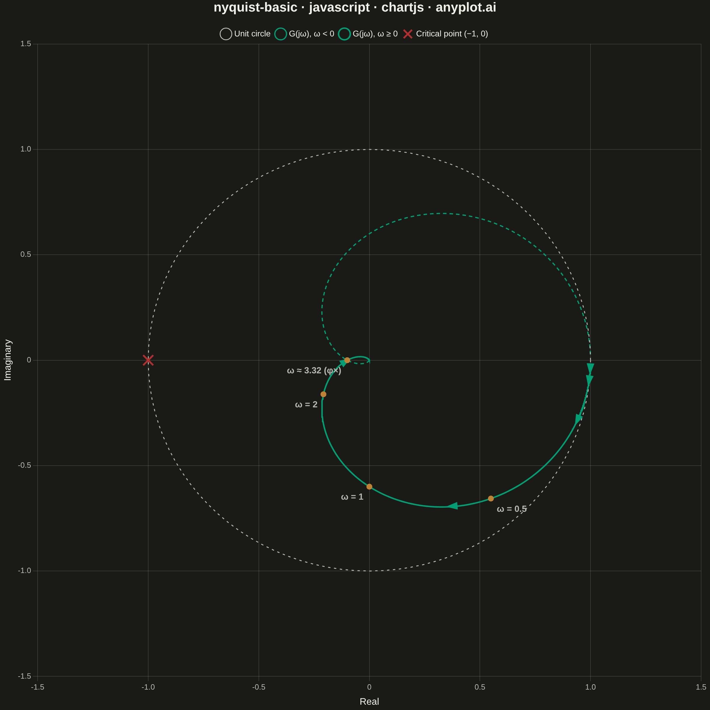
A Nyquist plot maps a system's open-loop frequency response onto the complex plane by plotting the imaginary part against the real part of the transfer function as frequency varies from zero to infinity. It is the primary tool for applying the Nyquist stability criterion to determine whether a closed-loop control system is stable. The plot visually reveals gain and phase margins and is widely used in classical control theory and electronic circuit design.
// anyplot.ai
// nyquist-basic: Nyquist Plot for Control Systems
// Library: chartjs 4.4.7 | JavaScript 22.22.3
// Quality: 84/100 | Created: 2026-06-17

//# anyplot-orientation: square

const t = window.ANYPLOT_TOKENS;

// --- Complex arithmetic ---
function cmul(a, b) { return { re: a.re * b.re - a.im * b.im, im: a.re * b.im + a.im * b.re }; }
function cdiv(a, b) {
  const d = b.re * b.re + b.im * b.im;
  return { re: (a.re * b.re + a.im * b.im) / d, im: (a.im * b.re - a.re * b.im) / d };
}

// G(s) = 6 / ((s+1)(s+2)(s+3)) — stable third-order plant
// DC gain = 1.0, phase crossover ω_pc ≈ 3.32 rad/s, gain margin = 10 (20 dB)
function evalG(w) {
  return cdiv(
    { re: 6, im: 0 },
    cmul(cmul({ re: 1, im: w }, { re: 2, im: w }), { re: 3, im: w })
  );
}

// --- Data ---
// 600 log-spaced frequencies: 0.01 to 100 rad/s
const N = 600;
const posFreqData = Array.from({ length: N }, (_, i) => {
  const w = Math.pow(10, -2 + (i * 4) / (N - 1));
  const G = evalG(w);
  return { x: G.re, y: G.im, w };
});
// Negative-frequency curve is the complex conjugate (mirror about real axis)
const negFreqData = [...posFreqData].reverse().map(p => ({ x: p.x, y: -p.y }));

// Unit circle for stability reference
const unitCircle = Array.from({ length: 101 }, (_, i) => {
  const theta = (2 * Math.PI * i) / 100;
  return { x: Math.cos(theta), y: Math.sin(theta) };
});

// Key frequency annotation points
const annotPts = [
  { w: 0.5,           label: "ω = 0.5"      },
  { w: 1.0,           label: "ω = 1"         },
  { w: 2.0,           label: "ω = 2"         },
  { w: Math.sqrt(11), label: "ω ≈ 3.32 (φ×)" },
].map(({ w, label }) => {
  const G = evalG(w);
  return { x: G.re, y: G.im, label };
});

// Indices along the positive-freq curve where direction arrows are drawn
const arrowIndices = [35, 100, 175, 265, 370];

// --- Background plugin ---
const bgPlugin = {
  id: "bg",
  beforeDraw(chart) {
    const ctx = chart.ctx;
    ctx.save();
    ctx.fillStyle = t.pageBg;
    ctx.fillRect(0, 0, chart.width, chart.height);
    ctx.restore();
  },
};

// --- Arrows + frequency-label plugin ---
const nyquistPlugin = {
  id: "nyquist",
  afterDraw(chart) {
    const ctx = chart.ctx;
    const xs = chart.scales.x;
    const ys = chart.scales.y;
    const toPx = (x, y) => ({ cx: xs.getPixelForValue(x), cy: ys.getPixelForValue(y) });

    ctx.save();

    // Direction arrows on positive-frequency curve
    ctx.fillStyle = t.palette[0];
    for (const idx of arrowIndices) {
      if (idx + 8 >= posFreqData.length) continue;
      const { cx: x0, cy: y0 } = toPx(posFreqData[idx].x, posFreqData[idx].y);
      const { cx: x1, cy: y1 } = toPx(posFreqData[idx + 8].x, posFreqData[idx + 8].y);
      const dx = x1 - x0, dy = y1 - y0;
      const len = Math.hypot(dx, dy);
      if (len < 1) continue;
      const nx = dx / len, ny = dy / len;
      const mx = (x0 + x1) / 2, my = (y0 + y1) / 2;
      const as = 13; // arrowhead half-size in logical canvas px
      ctx.beginPath();
      ctx.moveTo(mx + nx * as,                      my + ny * as);
      ctx.lineTo(mx - ny * (as * 0.5) - nx * (as * 0.5), my + nx * (as * 0.5) - ny * (as * 0.5));
      ctx.lineTo(mx + ny * (as * 0.5) - nx * (as * 0.5), my - nx * (as * 0.5) - ny * (as * 0.5));
      ctx.closePath();
      ctx.fill();
    }

    // Frequency annotation dots and labels
    ctx.font = "bold 15px sans-serif";
    for (const { x, y, label } of annotPts) {
      const { cx, cy } = toPx(x, y);
      // Ochre dot at the annotated point
      ctx.beginPath();
      ctx.arc(cx, cy, 5, 0, 2 * Math.PI);
      ctx.fillStyle = t.palette[3]; // Imprint ochre
      ctx.fill();
      // Label — offset away from curve
      const offX = x < 0.05 ? -10 : 10;
      const offY = y <= 0 ? 18 : -8;
      ctx.fillStyle = t.inkSoft;
      ctx.textAlign = x < 0.05 ? "right" : "left";
      ctx.textBaseline = "middle";
      ctx.fillText(label, cx + offX, cy + offY);
    }

    ctx.restore();
  },
};

// --- Mount ---
const canvas = document.createElement("canvas");
document.getElementById("container").appendChild(canvas);

// --- Chart ---
new Chart(canvas, {
  type: "scatter",
  data: {
    datasets: [
      {
        label: "Unit circle",
        data: unitCircle,
        borderColor: t.inkSoft,
        backgroundColor: "transparent",
        showLine: true,
        borderWidth: 1.5,
        borderDash: [4, 6],
        pointRadius: 0,
        tension: 0,
      },
      {
        label: "G(jω), ω < 0",
        data: negFreqData,
        borderColor: t.palette[0],
        backgroundColor: "transparent",
        showLine: true,
        borderWidth: 2,
        borderDash: [6, 5],
        pointRadius: 0,
        tension: 0,
      },
      {
        label: "G(jω), ω ≥ 0",
        data: posFreqData,
        borderColor: t.palette[0],
        backgroundColor: "transparent",
        showLine: true,
        borderWidth: 2.5,
        pointRadius: 0,
        tension: 0,
      },
      {
        label: "Critical point (−1, 0)",
        data: [{ x: -1, y: 0 }],
        borderColor: "#AE3030",
        backgroundColor: "#AE3030",
        pointStyle: "crossRot",
        pointRadius: 12,
        pointBorderWidth: 3,
        showLine: false,
      },
    ],
  },
  options: {
    responsive: true,
    maintainAspectRatio: false,
    animation: false,
    plugins: {
      title: {
        display: true,
        text: "nyquist-basic · javascript · chartjs · anyplot.ai",
        color: t.ink,
        font: { size: 22 },
        padding: { bottom: 14 },
      },
      legend: {
        labels: { color: t.ink, font: { size: 14 }, usePointStyle: true },
      },
      tooltip: { enabled: false },
    },
    scales: {
      x: {
        type: "linear",
        title: { display: true, text: "Real", color: t.ink, font: { size: 16 } },
        ticks: { color: t.inkSoft, font: { size: 13 } },
        grid: { color: t.grid },
        border: { display: false },
        min: -1.5,
        max: 1.5,
      },
      y: {
        type: "linear",
        title: { display: true, text: "Imaginary", color: t.ink, font: { size: 16 } },
        ticks: { color: t.inkSoft, font: { size: 13 } },
        grid: { color: t.grid },
        border: { display: false },
        min: -1.5,
        max: 1.5,
      },
    },
  },
  plugins: [bgPlugin, nyquistPlugin],
});
Runnable source as JSON, for any HTTP client: https://api.anyplot.ai/specs/nyquist-basic/chartjs/code. Any spec id and library id listed in llms-full.txt fit the same URL shape; every URL below is complete and callable.
{
  "spec_id": "nyquist-basic",
  "language": "javascript",
  "library": "chartjs",
  "page": "https://anyplot.ai/nyquist-basic/javascript/chartjs",
  "hub": "https://anyplot.ai/nyquist-basic",
  "code_json": "https://api.anyplot.ai/specs/nyquist-basic/chartjs/code",
  "spec_json": "https://api.anyplot.ai/specs/nyquist-basic",
  "render_light_png": "https://storage.googleapis.com/anyplot-images/plots/nyquist-basic/javascript/chartjs/plot-light.png",
  "render_dark_png": "https://storage.googleapis.com/anyplot-images/plots/nyquist-basic/javascript/chartjs/plot-dark.png",
  "interactive_light_html": "https://storage.googleapis.com/anyplot-images/plots/nyquist-basic/javascript/chartjs/plot-light.html",
  "interactive_dark_html": "https://storage.googleapis.com/anyplot-images/plots/nyquist-basic/javascript/chartjs/plot-dark.html",
  "quality_score": 84.0,
  "license": "MIT",
  "guide": "https://anyplot.ai/llms.txt"
}
Part of Nyquist Plot for Control Systems on anyplot.ai.