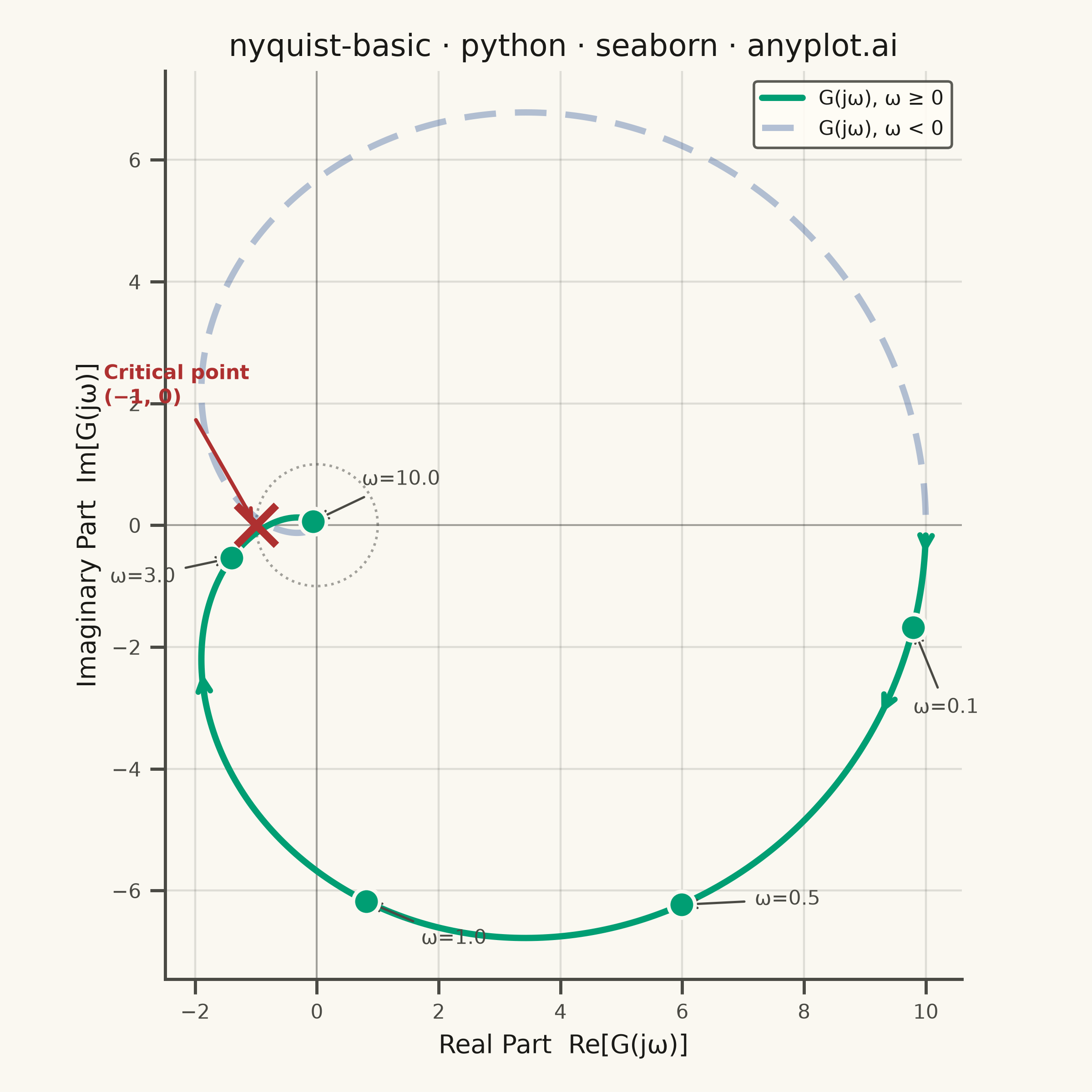
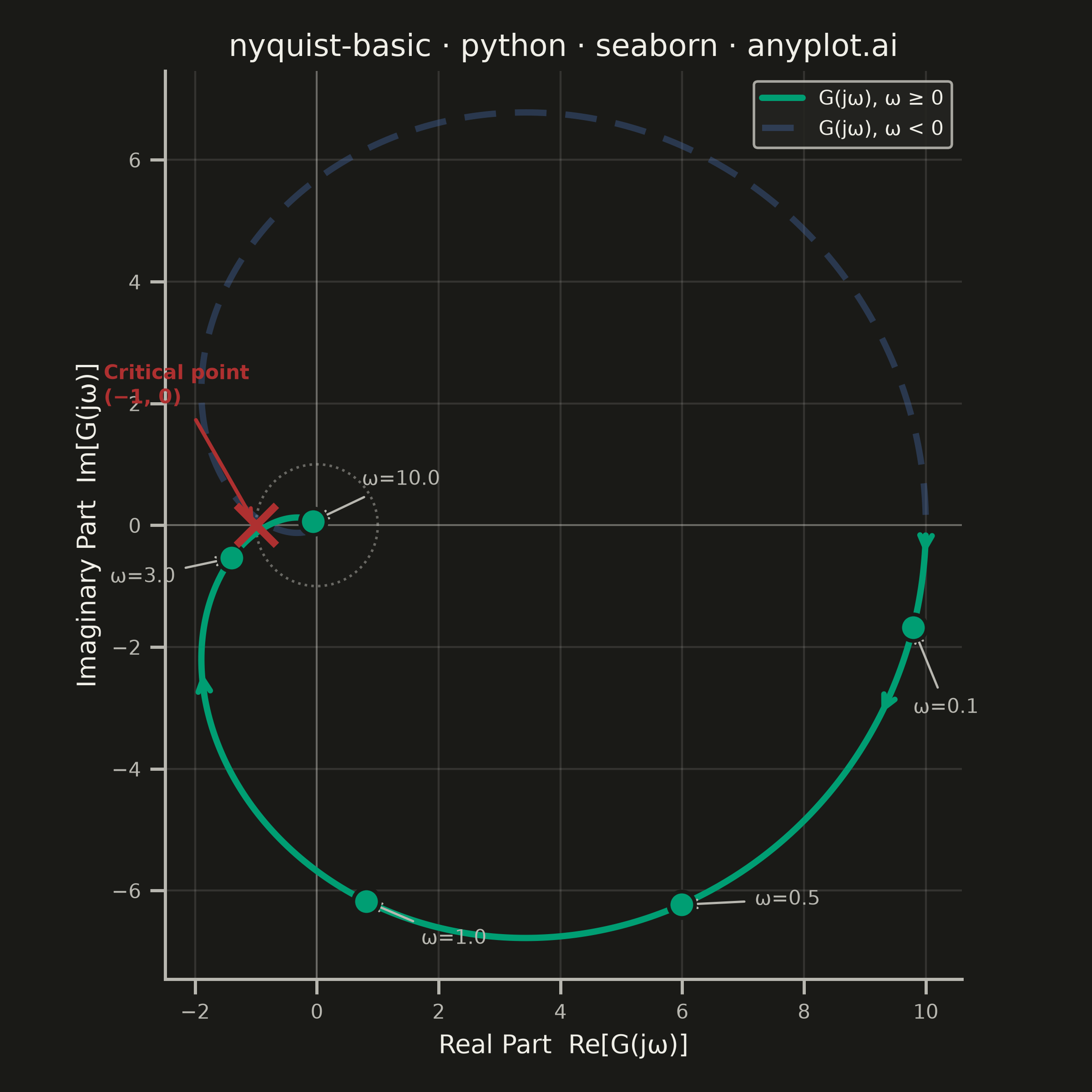
A Nyquist plot maps a system's open-loop frequency response onto the complex plane by plotting the imaginary part against the real part of the transfer function as frequency varies from zero to infinity. It is the primary tool for applying the Nyquist stability criterion to determine whether a closed-loop control system is stable. The plot visually reveals gain and phase margins and is widely used in classical control theory and electronic circuit design.
""" anyplot.ai
nyquist-basic: Nyquist Plot for Control Systems
Library: seaborn 0.13.2 | Python 3.13.13
Quality: 85/100 | Updated: 2026-06-17
"""

import os

import matplotlib.pyplot as plt
import numpy as np
import pandas as pd
import seaborn as sns
from scipy import signal


# Theme tokens
THEME = os.getenv("ANYPLOT_THEME", "light")
PAGE_BG = "#FAF8F1" if THEME == "light" else "#1A1A17"
ELEVATED_BG = "#FFFDF6" if THEME == "light" else "#242420"
INK = "#1A1A17" if THEME == "light" else "#F0EFE8"
INK_SOFT = "#4A4A44" if THEME == "light" else "#B8B7B0"

# Imprint palette — categorical positions
BRAND = "#009E73"  # position 1 — positive-frequency branch
IMPRINT_PURPLE = "#C475FD"  # position 2 — negative-frequency (mirror) branch
CRIT_RED = "#AE3030"  # semantic anchor — critical stability threshold

# Data — open-loop transfer function: G(s) = 10 / ((s+1)(0.5s+1)(0.2s+1))
num = [10.0]
den = np.polymul(np.polymul([1.0, 1.0], [0.5, 1.0]), [0.2, 1.0])
system = signal.TransferFunction(num, den)

omega = np.logspace(-2, 2, 800)
_, H = signal.freqresp(system, omega)

real_part = H.real
imag_part = H.imag

# Build DataFrame for seaborn-idiomatic plotting
df_pos = pd.DataFrame({"Real": real_part, "Imaginary": imag_part, "Branch": "G(jω), ω ≥ 0"})
df_neg = pd.DataFrame({"Real": real_part, "Imaginary": -imag_part, "Branch": "G(jω), ω < 0"})
df = pd.concat([df_pos, df_neg], ignore_index=True)

# Seaborn theme — ticks style with theme-adaptive chrome
sns.set_theme(
    style="ticks",
    rc={
        "figure.facecolor": PAGE_BG,
        "axes.facecolor": PAGE_BG,
        "axes.edgecolor": INK_SOFT,
        "axes.labelcolor": INK,
        "text.color": INK,
        "xtick.color": INK_SOFT,
        "ytick.color": INK_SOFT,
        "grid.color": INK,
        "grid.alpha": 0.12,
        "grid.linewidth": 0.8,
        "legend.facecolor": ELEVATED_BG,
        "legend.edgecolor": INK_SOFT,
    },
)

# Canvas — square 2400×2400 for equal-aspect Nyquist plot
fig, ax = plt.subplots(figsize=(6, 6), dpi=400)

# Both branches via seaborn lineplot with hue + dashes
sns.lineplot(
    data=df,
    x="Real",
    y="Imaginary",
    hue="Branch",
    palette=[BRAND, IMPRINT_PURPLE],
    linewidth=2.5,
    sort=False,
    estimator=None,
    style="Branch",
    dashes={"G(jω), ω ≥ 0": "", "G(jω), ω < 0": (5, 3)},
    ax=ax,
    legend=True,
)

# De-emphasize the mirror (negative-frequency) branch
for line in ax.get_lines():
    if line.get_linestyle() != "-":
        line.set_alpha(0.4)

# Unit circle for reference
theta = np.linspace(0, 2 * np.pi, 200)
ax.plot(np.cos(theta), np.sin(theta), color=INK_SOFT, linewidth=1.0, linestyle=":", alpha=0.5, zorder=1)

# Axis reference lines
ax.axhline(y=0, color=INK_SOFT, linewidth=0.7, zorder=0, alpha=0.4)
ax.axvline(x=0, color=INK_SOFT, linewidth=0.7, zorder=0, alpha=0.4)

# Critical point (−1, 0) — semantic red anchor marks instability threshold
ax.plot(-1, 0, marker="x", color=CRIT_RED, markersize=16, markeredgewidth=3, zorder=5)
ax.annotate(
    "Critical point\n(−1, 0)",
    xy=(-1, 0),
    xytext=(-1.8, 2.8),
    fontsize=8,
    color=CRIT_RED,
    fontweight="bold",
    arrowprops={"arrowstyle": "->", "color": CRIT_RED, "lw": 1.5},
)

# Direction arrows along positive-frequency branch
arrow_indices = [80, 250, 450]
for idx in arrow_indices:
    ax.annotate(
        "",
        xy=(real_part[idx + 8], imag_part[idx + 8]),
        xytext=(real_part[idx], imag_part[idx]),
        arrowprops={"arrowstyle": "->", "color": BRAND, "lw": 2.2},
    )

# Frequency annotations — spread offsets to minimise crowding near origin
freq_labels = [0.1, 0.5, 1.0, 3.0, 10.0]
freq_indices = [np.argmin(np.abs(omega - f)) for f in freq_labels]
freq_df = pd.DataFrame(
    {
        "Real": [real_part[i] for i in freq_indices],
        "Imaginary": [imag_part[i] for i in freq_indices],
        "Label": [f"ω={f}" for f in freq_labels],
    }
)

sns.scatterplot(
    data=freq_df,
    x="Real",
    y="Imaginary",
    color=BRAND,
    s=110,
    zorder=4,
    ax=ax,
    legend=False,
    edgecolor=PAGE_BG,
    linewidth=1.5,
)

# Text offsets chosen to spread labels away from crowded low-frequency region
offsets = {0.1: (0.0, -1.4), 0.5: (1.2, 0.0), 1.0: (0.9, -0.7), 3.0: (-2.0, -0.4), 10.0: (0.8, 0.6)}
for i, (_, row) in enumerate(freq_df.iterrows()):
    x, y = row["Real"], row["Imaginary"]
    f = freq_labels[i]
    ox, oy = offsets[f]
    ax.annotate(
        row["Label"],
        xy=(x, y),
        xytext=(x + ox, y + oy),
        fontsize=8,
        color=INK_SOFT,
        arrowprops={"arrowstyle": "->", "color": INK_SOFT, "lw": 0.9},
    )

# Style
title = "nyquist-basic · python · seaborn · anyplot.ai"
ax.set_title(title, fontsize=12, fontweight="medium", color=INK)
ax.set_xlabel("Real Part  Re[G(jω)]", fontsize=10, color=INK)
ax.set_ylabel("Imaginary Part  Im[G(jω)]", fontsize=10, color=INK)
ax.tick_params(axis="both", labelsize=8, colors=INK_SOFT)
ax.set_aspect("equal")
sns.despine(ax=ax)

# Grid — subtle both-axis for complex-plane orientation
ax.grid(True, alpha=0.12, linewidth=0.8, color=INK)

# Legend
handles, labels = ax.get_legend_handles_labels()
if handles:
    ax.legend(handles, labels, loc="upper right", framealpha=0.9, edgecolor=INK_SOFT, fontsize=8, facecolor=ELEVATED_BG)

plt.tight_layout()

# Save — no bbox_inches to preserve exact 2400×2400 canvas
plt.savefig(f"plot-{THEME}.png", dpi=400, facecolor=PAGE_BG)
Runnable source as JSON, for any HTTP client: https://api.anyplot.ai/specs/nyquist-basic/seaborn/code. Any spec id and library id listed in llms-full.txt fit the same URL shape; every URL below is complete and callable.
{
  "spec_id": "nyquist-basic",
  "language": "python",
  "library": "seaborn",
  "page": "https://anyplot.ai/nyquist-basic/python/seaborn",
  "hub": "https://anyplot.ai/nyquist-basic",
  "code_json": "https://api.anyplot.ai/specs/nyquist-basic/seaborn/code",
  "spec_json": "https://api.anyplot.ai/specs/nyquist-basic",
  "render_light_png": "https://storage.googleapis.com/anyplot-images/plots/nyquist-basic/python/seaborn/plot-light.png",
  "render_dark_png": "https://storage.googleapis.com/anyplot-images/plots/nyquist-basic/python/seaborn/plot-dark.png",
  "quality_score": 85.0,
  "license": "MIT",
  "guide": "https://anyplot.ai/llms.txt"
}
Part of Nyquist Plot for Control Systems on anyplot.ai.