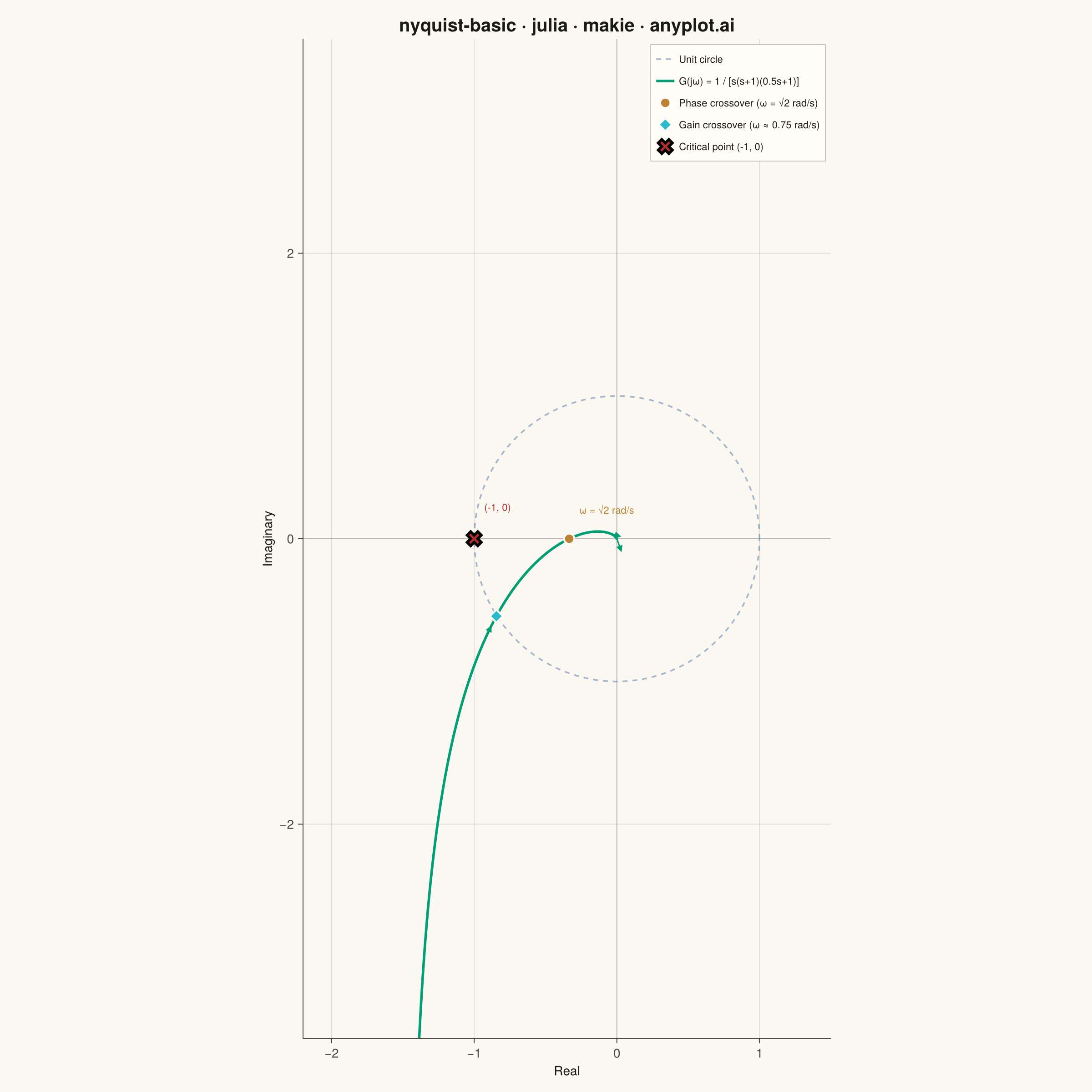
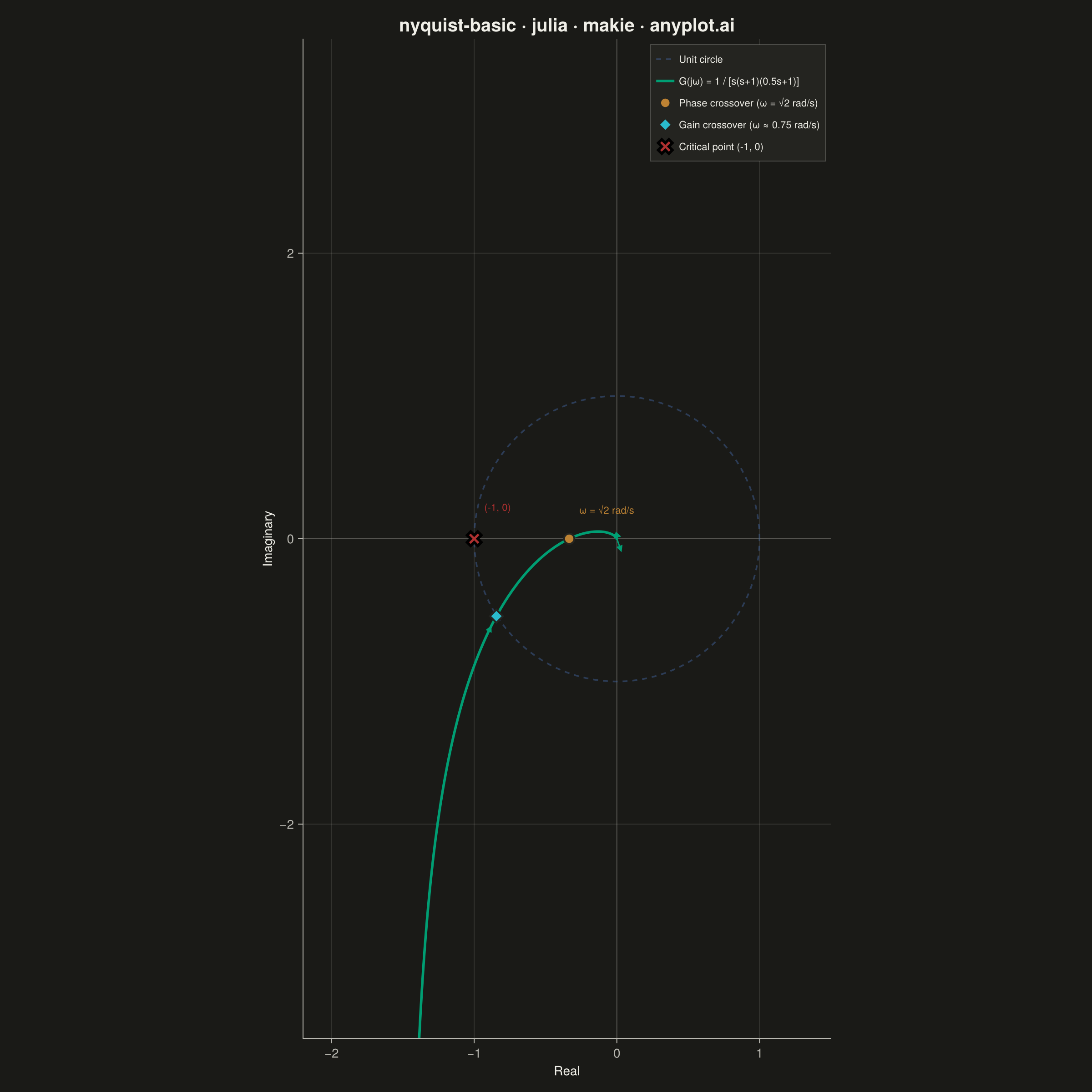
A Nyquist plot maps a system's open-loop frequency response onto the complex plane by plotting the imaginary part against the real part of the transfer function as frequency varies from zero to infinity. It is the primary tool for applying the Nyquist stability criterion to determine whether a closed-loop control system is stable. The plot visually reveals gain and phase margins and is widely used in classical control theory and electronic circuit design.
# anyplot.ai
# nyquist-basic: Nyquist Plot for Control Systems
# Library: makie 0.22.10 | Julia 1.11.9
# Quality: 89/100 | Created: 2026-06-17

using CairoMakie
using Colors
using Random

Random.seed!(42)

# Theme tokens
const THEME       = get(ENV, "ANYPLOT_THEME", "light")
const PAGE_BG     = THEME == "light" ? colorant"#FAF8F1" : colorant"#1A1A17"
const ELEVATED_BG = THEME == "light" ? colorant"#FFFDF6" : colorant"#242420"
const INK         = THEME == "light" ? colorant"#1A1A17" : colorant"#F0EFE8"
const INK_SOFT    = THEME == "light" ? colorant"#4A4A44" : colorant"#B8B7B0"

const IMPRINT_PALETTE = [
    colorant"#009E73",
    colorant"#C475FD",
    colorant"#4467A3",
    colorant"#BD8233",
    colorant"#AE3030",
    colorant"#2ABCCD",
    colorant"#954477",
    colorant"#99B314",
]

# Imprint sequential colormap: brand green → blue (for continuous frequency encoding)
const ANYPLOT_SEQ = cgrad([colorant"#009E73", colorant"#4467A3"])

# Frequency response: G(s) = 1 / (s(s+1)(0.5s+1))
# Phase crossover at ω_pc = √2 rad/s → G(jω_pc) = -1/3 → gain margin = 3
n_points = 800
ω = 10 .^ range(log10(0.04), log10(100.0), length=n_points)
G_jω = [1.0 / (im * w * (1 + im * w) * (1 + 0.5 * im * w)) for w in ω]

re_vals = real.(G_jω)
im_vals = imag.(G_jω)

# Gain crossover (|G| = 1) and phase crossover (phase = -180°)
mag = abs.(G_jω)
gc_idx = argmin(abs.(mag .- 1.0))
ω_gc_val = ω[gc_idx]
G_gc = G_jω[gc_idx]
phase_margin_deg = 180.0 + angle(G_gc) * (180.0 / π)

ph_deg = angle.(G_jω) .* (180.0 / π)
pc_idx = argmin(abs.(ph_deg .+ 180.0))
G_pc   = G_jω[pc_idx]
gain_margin = round(1.0 / abs(G_pc); digits=1)

# Log-frequency for continuous color encoding along the Nyquist curve
log_ω = log10.(ω)
log_ω_min, log_ω_max = extrema(log_ω)

# Unit circle
θ_circle = range(0.0, 2π, length=300)

# Figure — square canvas for 1:1 aspect (2400×2400 output at px_per_unit=2)
fig = Figure(
    size            = (1200, 1200),
    fontsize        = 14,
    backgroundcolor = PAGE_BG,
)

ink_r = Float32(INK.r)
ink_g = Float32(INK.g)
ink_b = Float32(INK.b)

title_str  = "nyquist-basic · julia · makie · anyplot.ai"
n_title    = length(title_str)
title_size = n_title > 67 ? round(Int, 20 * 67 / n_title) : 20

ax = Axis(
    fig[1, 1];
    title              = title_str,
    titlesize          = title_size,
    titlecolor         = INK,
    xlabel             = "Real",
    ylabel             = "Imaginary",
    xlabelsize         = 14,
    ylabelsize         = 14,
    xlabelcolor        = INK,
    ylabelcolor        = INK,
    xticklabelcolor    = INK_SOFT,
    yticklabelcolor    = INK_SOFT,
    xticklabelsize     = 12,
    yticklabelsize     = 12,
    xtickcolor         = INK_SOFT,
    ytickcolor         = INK_SOFT,
    backgroundcolor    = PAGE_BG,
    topspinevisible    = false,
    rightspinevisible  = false,
    leftspinecolor     = INK_SOFT,
    bottomspinecolor   = INK_SOFT,
    xgridcolor         = RGBAf(ink_r, ink_g, ink_b, 0.12f0),
    ygridcolor         = RGBAf(ink_r, ink_g, ink_b, 0.12f0),
    aspect             = DataAspect(),
)

# Reference lines through origin
hlines!(ax, [0.0]; color = (INK_SOFT, 0.25), linewidth = 1.0)
vlines!(ax, [0.0]; color = (INK_SOFT, 0.25), linewidth = 1.0)

# Unit circle reference
lines!(ax, cos.(θ_circle), sin.(θ_circle);
    color     = (IMPRINT_PALETTE[3], 0.45),
    linewidth = 1.8,
    linestyle = :dash,
    label     = "Unit circle",
)

# Nyquist curve — colored by log₁₀(ω) using Imprint sequential colormap
# Low frequency (ω → 0) renders in brand green; high frequency in blue
lines!(ax, re_vals, im_vals;
    color      = log_ω,
    colormap   = ANYPLOT_SEQ,
    colorrange = (log_ω_min, log_ω_max),
    linewidth  = 2.8,
    label      = "G(jω) = 1 / [s(s+1)(0.5s+1)]",
)

# Direction arrows showing increasing-frequency direction
for idx in [80, 260, 460]
    if idx + 4 <= length(re_vals)
        dx = re_vals[idx + 4] - re_vals[idx]
        dy = im_vals[idx + 4] - im_vals[idx]
        nd = sqrt(dx^2 + dy^2)
        if nd > 1e-10
            u = dx / nd * 0.07
            v = dy / nd * 0.07
            arrows!(ax,
                [re_vals[idx]], [im_vals[idx]],
                [u], [v];
                arrowsize  = 10,
                arrowcolor = INK_SOFT,
                linecolor  = INK_SOFT,
                linewidth  = 1.5,
            )
        end
    end
end

# Phase crossover marker
scatter!(ax, [real(G_pc)], [imag(G_pc)];
    color       = IMPRINT_PALETTE[4],
    markersize  = 16,
    marker      = :circle,
    strokewidth = 2,
    strokecolor = ELEVATED_BG,
    label       = "Phase crossover (ω = √2 rad/s)",
)

# Gain crossover marker
scatter!(ax, [real(G_gc)], [imag(G_gc)];
    color       = IMPRINT_PALETTE[6],
    markersize  = 16,
    marker      = :diamond,
    strokewidth = 2,
    strokecolor = ELEVATED_BG,
    label       = "Gain crossover (ω ≈ $(round(ω_gc_val; digits=2)) rad/s)",
)

# Critical point (-1, 0)
scatter!(ax, [-1.0], [0.0];
    color       = IMPRINT_PALETTE[5],
    markersize  = 22,
    marker      = :xcross,
    strokewidth = 3,
    label       = "Critical point (-1, 0)",
)

# Gain margin: dotted line from phase crossover point to critical point
lines!(ax, [real(G_pc), -1.0], [0.0, 0.0];
    color     = (INK_SOFT, 0.45),
    linewidth = 1.8,
    linestyle = :dot,
)
text!(ax, (real(G_pc) + (-1.0)) / 2, 0.13;
    text     = "GM = $(gain_margin)",
    color    = INK_SOFT,
    fontsize = 11,
    align    = (:center, :bottom),
)

# Frequency annotations
text!(ax, real(G_pc) + 0.07, imag(G_pc) + 0.16;
    text     = "ω = √2 rad/s",
    color    = IMPRINT_PALETTE[4],
    fontsize = 11,
)
text!(ax, -1.0 + 0.07, 0.22;
    text     = "(-1, 0)",
    color    = IMPRINT_PALETTE[5],
    fontsize = 11,
)
text!(ax, real(G_gc) - 0.10, imag(G_gc) - 0.28;
    text     = "PM ≈ $(round(Int, phase_margin_deg))°",
    color    = IMPRINT_PALETTE[6],
    fontsize = 11,
    align    = (:right, :top),
)

xlims!(ax, -2.2, 1.5)
ylims!(ax, -4.0, 2.0)

axislegend(ax;
    position        = :rt,
    backgroundcolor = ELEVATED_BG,
    framecolor      = (INK_SOFT, 0.3),
    labelsize       = 11,
    labelcolor      = INK,
    rowgap          = 4,
)

# Colorbar: maps log₁₀(ω) to the Imprint sequential gradient — Makie layout element
Colorbar(fig[1, 2];
    colormap       = ANYPLOT_SEQ,
    limits         = (log_ω_min, log_ω_max),
    label          = "log₁₀(ω)  [rad/s]",
    labelsize      = 13,
    labelcolor     = INK,
    ticklabelsize  = 11,
    ticklabelcolor = INK_SOFT,
    tickcolor      = INK_SOFT,
    width          = 18,
)

# Stability summary — Makie Label layout element below the plot
stability_str = "System: STABLE  ·  Gain Margin = $(gain_margin)  ·  Phase Margin ≈ $(round(Int, phase_margin_deg))°"
Label(fig[2, 1:2], stability_str;
    fontsize  = 12,
    color     = INK_SOFT,
    halign    = :left,
    tellwidth = false,
    padding   = (8, 0, 4, 4),
)

save("plot-$(THEME).png", fig; px_per_unit = 2)
Runnable source as JSON, for any HTTP client: https://api.anyplot.ai/specs/nyquist-basic/makie/code. Any spec id and library id listed in llms-full.txt fit the same URL shape; every URL below is complete and callable.
{
  "spec_id": "nyquist-basic",
  "language": "julia",
  "library": "makie",
  "page": "https://anyplot.ai/nyquist-basic/julia/makie",
  "hub": "https://anyplot.ai/nyquist-basic",
  "code_json": "https://api.anyplot.ai/specs/nyquist-basic/makie/code",
  "spec_json": "https://api.anyplot.ai/specs/nyquist-basic",
  "render_light_png": "https://storage.googleapis.com/anyplot-images/plots/nyquist-basic/julia/makie/plot-light.png",
  "render_dark_png": "https://storage.googleapis.com/anyplot-images/plots/nyquist-basic/julia/makie/plot-dark.png",
  "quality_score": 89.0,
  "license": "MIT",
  "guide": "https://anyplot.ai/llms.txt"
}
Part of Nyquist Plot for Control Systems on anyplot.ai.