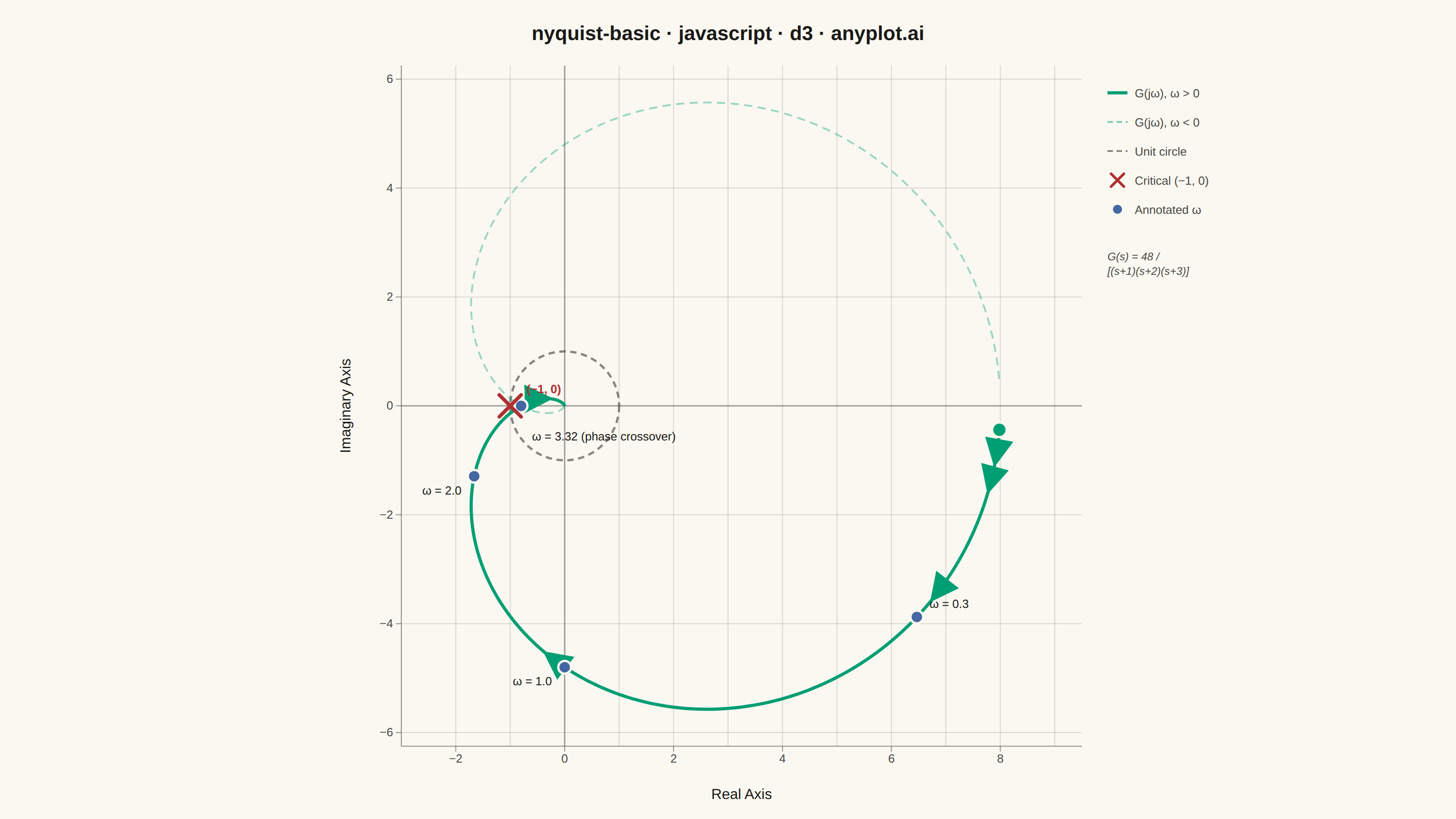
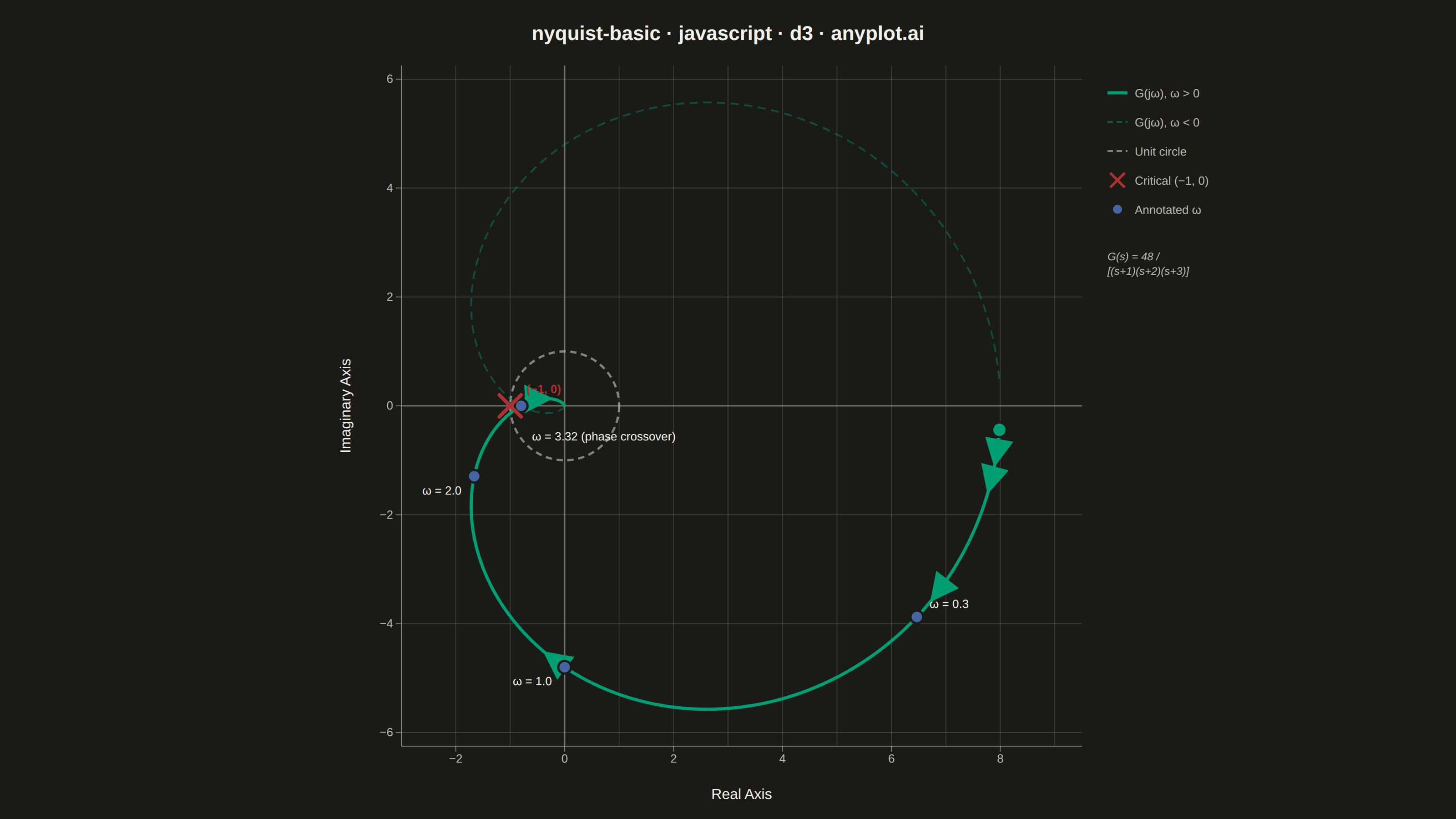
A Nyquist plot maps a system's open-loop frequency response onto the complex plane by plotting the imaginary part against the real part of the transfer function as frequency varies from zero to infinity. It is the primary tool for applying the Nyquist stability criterion to determine whether a closed-loop control system is stable. The plot visually reveals gain and phase margins and is widely used in classical control theory and electronic circuit design.
// anyplot.ai
// nyquist-basic: Nyquist Plot for Control Systems
// Library: d3 7.9.0 | JavaScript 22.22.3
// Quality: 88/100 | Created: 2026-06-17

const t = window.ANYPLOT_TOKENS;
const { width, height } = window.ANYPLOT_SIZE;

// G(s) = 48/((s+1)(s+2)(s+3)): Re[G(jω)] = 48rd/d², Im[G(jω)] = −48id/d²
// where rd = 6−6ω², id = ω(11−ω²), d² = rd²+id²

// 600 log-spaced frequencies ω ∈ [0.03, 30]
const N = 600;
const wMin = 0.03, wMax = 30;
const omegas = Array.from({ length: N }, (_, i) =>
  wMin * Math.pow(wMax / wMin, i / (N - 1))
);
const pos = omegas.map((w) => {
  const rd = 6 - 6 * w * w, id = w * (11 - w * w), d2 = rd * rd + id * id;
  return { re: 48 * rd / d2, im: -48 * id / d2, w };
});
// Negative-frequency mirror: reflect Im across real axis, reverse so it joins at ω→−∞
const neg = [...pos].reverse().map((p) => ({ re: p.re, im: -p.im }));

// Layout — square inner plot centred in landscape canvas
const margin = { top: 72, right: 50, bottom: 80, left: 80 };
const iw = width  - margin.left - margin.right;
const ih = height - margin.top  - margin.bottom;
const ps = Math.min(iw, ih); // square side (height-limited: 748 px at 1600×900)
const ox = margin.left + (iw - ps) / 2; // left edge of square plot
const oy = margin.top;                   // top  edge of square plot

// Equal-range scales for 1:1 aspect ratio — unit circle stays circular
const domRange = 12.5;
const xMid = 3.25, yMid = 0;
const xDom = [xMid - domRange / 2, xMid + domRange / 2]; // [−3, 9.5]
const yDom = [yMid - domRange / 2, yMid + domRange / 2]; // [−6.25, 6.25]
const xSc  = d3.scaleLinear().domain(xDom).range([0, ps]);
const ySc  = d3.scaleLinear().domain(yDom).range([ps, 0]);

// SVG root
const svg = d3.select("#container").append("svg")
  .attr("width", width).attr("height", height);

// Defs: clip path + arrow marker
const defs = svg.append("defs");
defs.append("clipPath").attr("id", "nyq-clip")
  .append("rect").attr("width", ps).attr("height", ps);
defs.append("marker")
  .attr("id", "arr")
  .attr("viewBox", "0 -5 10 10")
  .attr("refX", 8).attr("refY", 0)
  .attr("markerWidth", 7).attr("markerHeight", 7)
  .attr("orient", "auto")
  .append("path").attr("d", "M0,-5L10,0L0,5Z")
  .attr("fill", t.palette[0]);

const root = svg.append("g").attr("transform", `translate(${ox},${oy})`);

// Plot area background must come BEFORE the clipped group so it stays behind the data
root.append("rect").attr("width", ps).attr("height", ps)
  .attr("fill", t.pageBg);

const clipped = root.append("g").attr("clip-path", "url(#nyq-clip)");

// Grid lines
[-3,-2,-1,0,1,2,3,4,5,6,7,8,9].forEach((v) => {
  clipped.append("line")
    .attr("x1", xSc(v)).attr("x2", xSc(v)).attr("y1", 0).attr("y2", ps)
    .attr("stroke", t.grid).attr("stroke-width", 1);
});
[-6,-4,-2,0,2,4,6].forEach((v) => {
  clipped.append("line")
    .attr("x1", 0).attr("x2", ps).attr("y1", ySc(v)).attr("y2", ySc(v))
    .attr("stroke", t.grid).attr("stroke-width", 1);
});

// Zero-axes (real and imaginary)
clipped.append("line")
  .attr("x1", 0).attr("x2", ps).attr("y1", ySc(0)).attr("y2", ySc(0))
  .attr("stroke", t.inkSoft).attr("stroke-width", 1.5).attr("opacity", 0.45);
clipped.append("line")
  .attr("x1", xSc(0)).attr("x2", xSc(0)).attr("y1", 0).attr("y2", ps)
  .attr("stroke", t.inkSoft).attr("stroke-width", 1.5).attr("opacity", 0.45);

// Unit circle (dashed reference)
clipped.append("circle")
  .attr("cx", xSc(0)).attr("cy", ySc(0))
  .attr("r", xSc(1) - xSc(0))
  .attr("fill", "none")
  .attr("stroke", t.inkSoft).attr("stroke-width", 2.5)
  .attr("stroke-dasharray", "7,5").attr("opacity", 0.65);

// Line generator
const lineGen = d3.line().x((d) => xSc(d.re)).y((d) => ySc(d.im));

// Mirror curve — ω < 0 (dashed, semi-transparent)
clipped.append("path")
  .datum(neg)
  .attr("fill", "none")
  .attr("stroke", t.palette[0])
  .attr("stroke-width", 2)
  .attr("stroke-dasharray", "9,6")
  .attr("opacity", 0.38)
  .attr("d", lineGen);

// Main curve — ω > 0 (solid)
clipped.append("path")
  .datum(pos)
  .attr("fill", "none")
  .attr("stroke", t.palette[0])
  .attr("stroke-width", 3.5)
  .attr("d", lineGen);

// Direction arrows showing increasing frequency
[70, 105, 185, 305, 435].forEach((i) => {
  if (i + 4 >= pos.length) return;
  const p1 = pos[i], p2 = pos[i + 4];
  clipped.append("line")
    .attr("x1", xSc(p1.re)).attr("y1", ySc(p1.im))
    .attr("x2", xSc(p2.re)).attr("y2", ySc(p2.im))
    .attr("stroke", t.palette[0]).attr("stroke-width", 4.5)
    .attr("marker-end", "url(#arr)");
});

// Frequency-annotation dots and labels
// Key ω values: 0.3, 1.0, 2.0, √11 (phase crossover)
const phaseXover = Math.sqrt(11); // ≈ 3.317 rad/s
const annotPts = [
  { omega: 0.3,         label: "ω = 0.3",                   dx:  14, dy: -10, anchor: "start" },
  { omega: 1.0,         label: "ω = 1.0",                   dx: -14, dy:  20, anchor: "end"   },
  { omega: 2.0,         label: "ω = 2.0",                   dx: -14, dy:  20, anchor: "end"   },
  { omega: phaseXover,  label: "ω = 3.32 (phase crossover)", dx:  12, dy:  38, anchor: "start" },
];
annotPts.forEach(({ omega, label, dx, dy, anchor }) => {
  const rd = 6 - 6 * omega * omega, id = omega * (11 - omega * omega), d2 = rd * rd + id * id;
  const p = { re: 48 * rd / d2, im: -48 * id / d2 };
  clipped.append("circle")
    .attr("cx", xSc(p.re)).attr("cy", ySc(p.im)).attr("r", 7)
    .attr("fill", t.palette[2]).attr("stroke", t.pageBg).attr("stroke-width", 2.5);
  clipped.append("text")
    .attr("x", xSc(p.re) + dx).attr("y", ySc(p.im) + dy)
    .attr("fill", t.ink).style("font-size", "13px").style("font-weight", "500")
    .attr("text-anchor", anchor)
    .text(label);
});

// Critical point (−1, 0) — red × marker
const cpx = xSc(-1), cpy = ySc(0), cs = 12;
[[-cs,-cs,cs,cs],[cs,-cs,-cs,cs]].forEach(([x1,y1,x2,y2]) => {
  clipped.append("line")
    .attr("x1", cpx + x1).attr("y1", cpy + y1)
    .attr("x2", cpx + x2).attr("y2", cpy + y2)
    .attr("stroke", "#AE3030").attr("stroke-width", 4)
    .attr("stroke-linecap", "round");
});
clipped.append("text")
  .attr("x", cpx + 18).attr("y", cpy - 14)
  .attr("fill", "#AE3030").style("font-size", "13px").style("font-weight", "600")
  .attr("text-anchor", "start")
  .text("(−1, 0)");

// Starting-point dot (DC gain: ω → 0⁺)
clipped.append("circle")
  .attr("cx", xSc(pos[0].re)).attr("cy", ySc(pos[0].im)).attr("r", 8)
  .attr("fill", t.palette[0]).attr("stroke", t.pageBg).attr("stroke-width", 2.5);

// Axes
const xAxisG = root.append("g").attr("transform", `translate(0,${ps})`).call(
  d3.axisBottom(xSc).ticks(8).tickSizeOuter(0)
);
const yAxisG = root.append("g").call(
  d3.axisLeft(ySc).ticks(7).tickSizeOuter(0)
);
for (const ax of [xAxisG, yAxisG]) {
  ax.selectAll("text").attr("fill", t.inkSoft).style("font-size", "13px");
  ax.selectAll("line").attr("stroke", t.inkSoft).attr("opacity", 0.6);
  ax.select(".domain").attr("stroke", t.inkSoft).attr("opacity", 0.6);
}

// Axis labels
root.append("text")
  .attr("x", ps / 2).attr("y", ps + 58)
  .attr("text-anchor", "middle").attr("fill", t.ink)
  .style("font-size", "16px").style("font-weight", "500")
  .text("Real Axis");

root.append("text")
  .attr("transform", `translate(-56,${ps / 2}) rotate(-90)`)
  .attr("text-anchor", "middle").attr("fill", t.ink)
  .style("font-size", "16px").style("font-weight", "500")
  .text("Imaginary Axis");

// Legend (right of square plot)
const lx  = ox + ps + 28;
const ly0 = oy + 30;
const legendItems = [
  { color: t.palette[0], label: "G(jω), ω > 0", solid: true,  opacity: 1    },
  { color: t.palette[0], label: "G(jω), ω < 0", solid: false, opacity: 0.5  },
  { color: t.inkSoft,    label: "Unit circle",             solid: false, opacity: 0.65 },
  { color: "#AE3030",    label: "Critical (−1, 0)",   type: "x"                   },
  { color: t.palette[2], label: "Annotated ω",        type: "dot"                 },
];
legendItems.forEach(({ color, label, solid, opacity, type }, i) => {
  const ly = ly0 + i * 32;
  if (type === "x") {
    const cx2 = lx + 11, cy2 = ly;
    [[-7,-7,7,7],[7,-7,-7,7]].forEach(([x1,y1,x2,y2]) => {
      svg.append("line")
        .attr("x1", cx2+x1).attr("y1", cy2+y1)
        .attr("x2", cx2+x2).attr("y2", cy2+y2)
        .attr("stroke", color).attr("stroke-width", 3).attr("stroke-linecap", "round");
    });
  } else if (type === "dot") {
    svg.append("circle").attr("cx", lx + 11).attr("cy", ly).attr("r", 6)
      .attr("fill", color).attr("stroke", t.pageBg).attr("stroke-width", 2);
  } else {
    const leg = svg.append("line")
      .attr("x1", lx).attr("y1", ly).attr("x2", lx + 22).attr("y2", ly)
      .attr("stroke", color).attr("stroke-width", solid ? 3.5 : 2)
      .attr("opacity", opacity);
    if (!solid) leg.attr("stroke-dasharray", "6,4");
  }
  svg.append("text").attr("x", lx + 30).attr("y", ly + 5)
    .attr("fill", t.inkSoft).style("font-size", "13px")
    .text(label);
});

// Transfer function note below legend
svg.append("text")
  .attr("x", lx).attr("y", ly0 + legendItems.length * 32 + 24)
  .attr("fill", t.inkSoft).style("font-size", "12px").style("font-style", "italic")
  .text("G(s) = 48 /");
svg.append("text")
  .attr("x", lx).attr("y", ly0 + legendItems.length * 32 + 40)
  .attr("fill", t.inkSoft).style("font-size", "12px").style("font-style", "italic")
  .text("[(s+1)(s+2)(s+3)]");

// Title
svg.append("text")
  .attr("x", width / 2).attr("y", 44)
  .attr("text-anchor", "middle").attr("fill", t.ink)
  .style("font-size", "22px").style("font-weight", "600")
  .text("nyquist-basic · javascript · d3 · anyplot.ai");
Runnable source as JSON, for any HTTP client: https://api.anyplot.ai/specs/nyquist-basic/d3/code. Any spec id and library id listed in llms-full.txt fit the same URL shape; every URL below is complete and callable.
{
  "spec_id": "nyquist-basic",
  "language": "javascript",
  "library": "d3",
  "page": "https://anyplot.ai/nyquist-basic/javascript/d3",
  "hub": "https://anyplot.ai/nyquist-basic",
  "code_json": "https://api.anyplot.ai/specs/nyquist-basic/d3/code",
  "spec_json": "https://api.anyplot.ai/specs/nyquist-basic",
  "render_light_png": "https://storage.googleapis.com/anyplot-images/plots/nyquist-basic/javascript/d3/plot-light.png",
  "render_dark_png": "https://storage.googleapis.com/anyplot-images/plots/nyquist-basic/javascript/d3/plot-dark.png",
  "interactive_light_html": "https://storage.googleapis.com/anyplot-images/plots/nyquist-basic/javascript/d3/plot-light.html",
  "interactive_dark_html": "https://storage.googleapis.com/anyplot-images/plots/nyquist-basic/javascript/d3/plot-dark.html",
  "quality_score": 88.0,
  "license": "MIT",
  "guide": "https://anyplot.ai/llms.txt"
}
Part of Nyquist Plot for Control Systems on anyplot.ai.