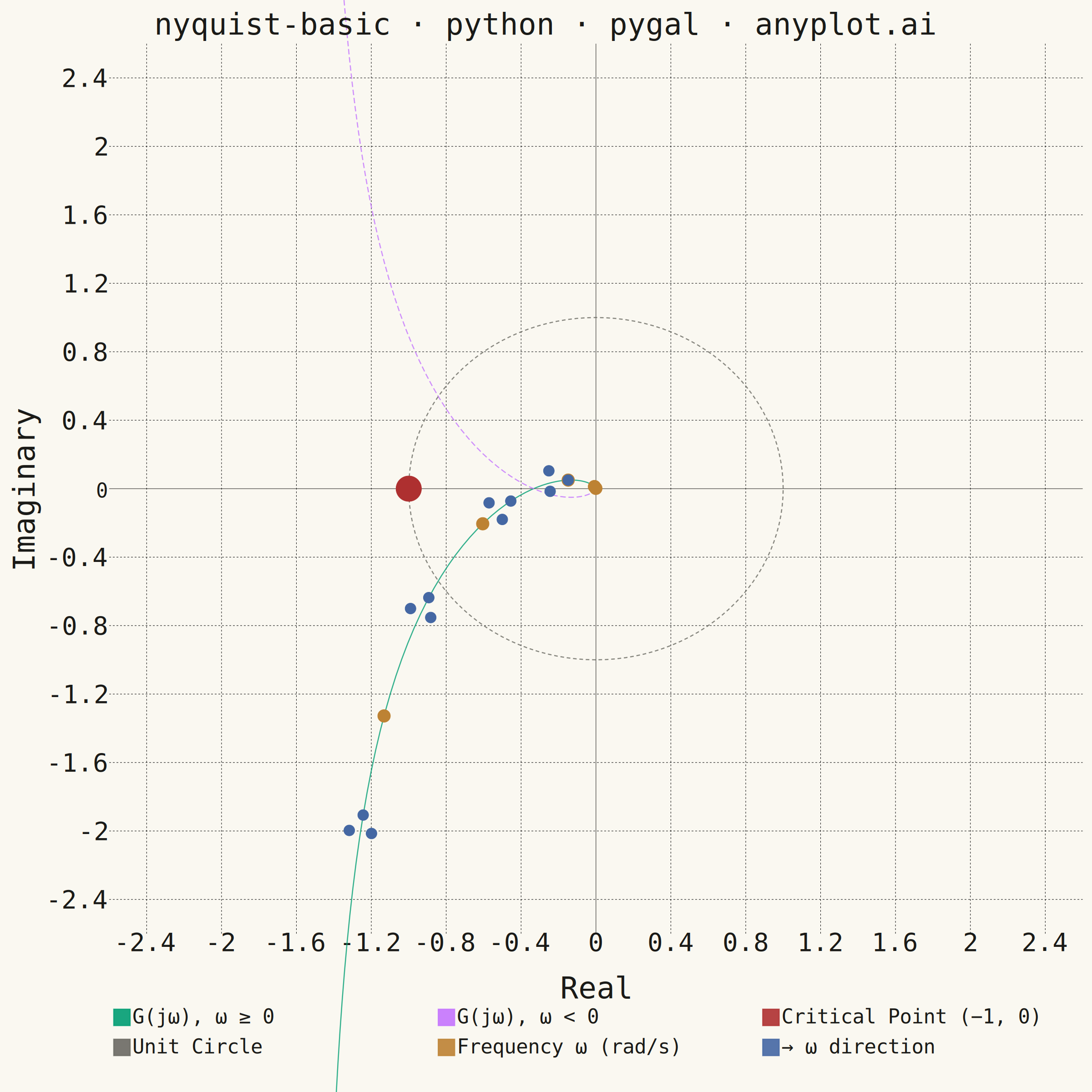
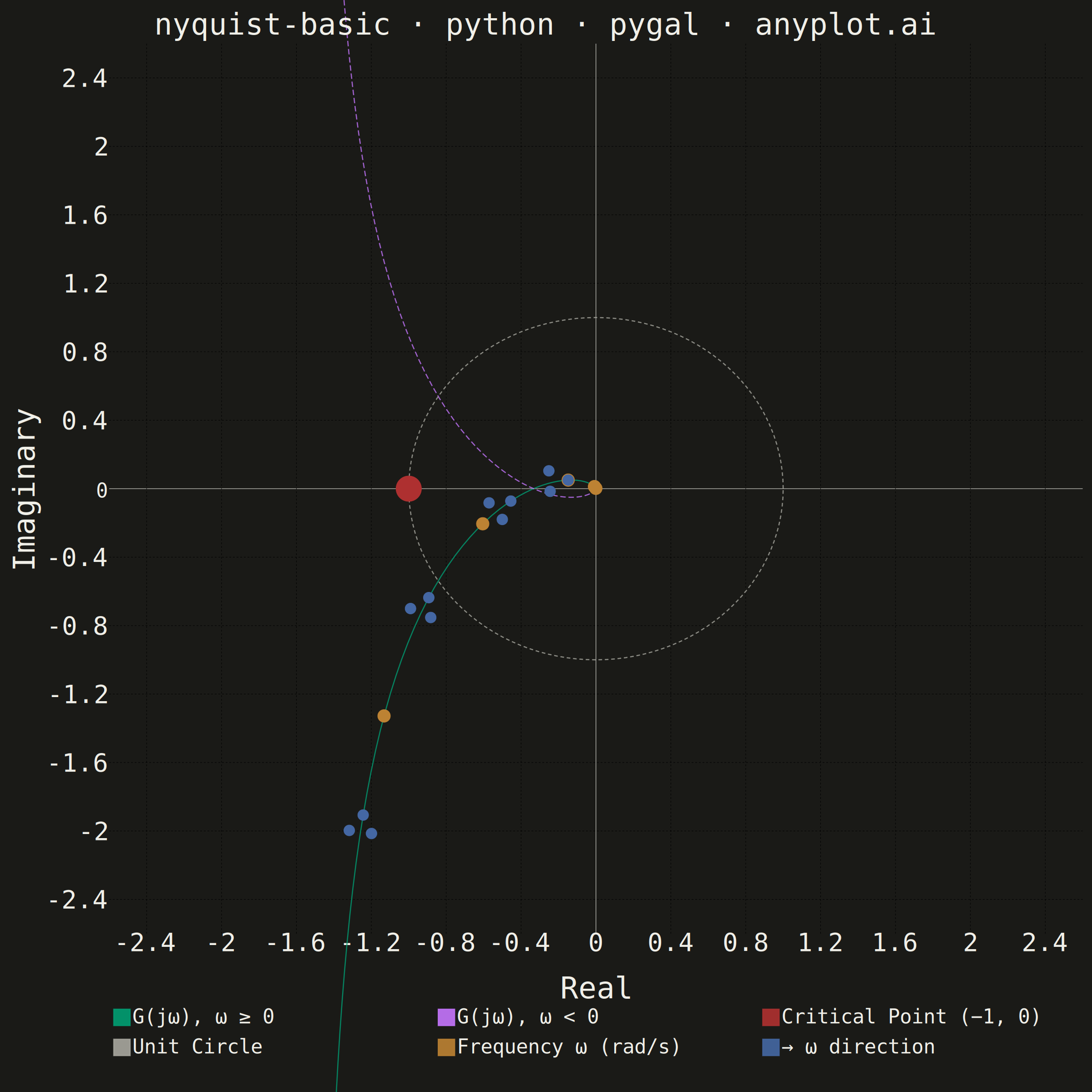
A Nyquist plot maps a system's open-loop frequency response onto the complex plane by plotting the imaginary part against the real part of the transfer function as frequency varies from zero to infinity. It is the primary tool for applying the Nyquist stability criterion to determine whether a closed-loop control system is stable. The plot visually reveals gain and phase margins and is widely used in classical control theory and electronic circuit design.
""" anyplot.ai
nyquist-basic: Nyquist Plot for Control Systems
Library: pygal 3.1.0 | Python 3.13.14
Quality: 82/100 | Updated: 2026-06-17
"""

import math
import os

import numpy as np
import pygal
from pygal.style import Style


# Theme tokens
THEME = os.getenv("ANYPLOT_THEME", "light")
PAGE_BG = "#FAF8F1" if THEME == "light" else "#1A1A17"
INK = "#1A1A17" if THEME == "light" else "#F0EFE8"
INK_MUTED = "#6B6A63" if THEME == "light" else "#A8A79F"

# Imprint palette — canonical order; semantic exceptions noted
# Critical point gets semantic red (#AE3030) — valid danger/critical exception
CHART_COLORS = (
    "#009E73",  # Imprint pos 1 — positive frequency curve
    "#C475FD",  # Imprint pos 2 — negative frequency curve (canonical order)
    "#AE3030",  # Semantic red — critical point (danger marker exception)
    INK_MUTED,  # Muted anchor — unit circle (reference element, not categorical)
    "#BD8233",  # Imprint pos 4 — frequency annotation markers
    "#4467A3",  # Imprint pos 3 — direction arrows
)

# Data — Transfer function G(s) = 2 / [s(s+1)(s+2)]
omega = np.logspace(-2, 2, 800)
s = 1j * omega
G = 2.0 / (s * (s + 1) * (s + 2))

real_part = G.real
imag_part = G.imag

# Mirror for negative frequencies (Nyquist contour reflection)
real_mirror = real_part[::-1]
imag_mirror = -imag_part[::-1]

# Title
title = "nyquist-basic · python · pygal · anyplot.ai"
title_len = len(title)
base_fontsize = 66
title_fontsize = round(base_fontsize * 67 / title_len) if title_len > 67 else base_fontsize

# Style — canonical pygal sizing for 2400×2400 square canvas
custom_style = Style(
    background=PAGE_BG,
    plot_background=PAGE_BG,
    foreground=INK,
    foreground_strong=INK,
    foreground_subtle=INK_MUTED,
    colors=CHART_COLORS,
    title_font_size=title_fontsize,
    label_font_size=56,
    major_label_font_size=44,
    legend_font_size=44,
    value_font_size=36,
    stroke_width=2.5,
    opacity=0.9,
    opacity_hover=0.95,
)

# Chart — square 2400×2400 (spec requires 1:1 aspect ratio for unit circle)
chart = pygal.XY(
    width=2400,
    height=2400,
    style=custom_style,
    title=title,
    x_title="Real",
    y_title="Imaginary",
    show_legend=True,
    legend_at_bottom=True,
    legend_box_size=36,
    dots_size=3,
    stroke=True,
    show_x_guides=True,
    show_y_guides=True,
    explicit_size=True,
    range=(-2.5, 2.5),
    xrange=(-2.5, 2.5),
)

# Positive frequency curve (main)
step = 4
nyquist_positive = [
    {"value": (float(real_part[i]), float(imag_part[i])), "label": f"ω = {omega[i]:.3f} rad/s"}
    for i in range(0, len(omega), step)
]
chart.add("G(jω), ω ≥ 0", nyquist_positive, show_dots=False, stroke_style={"width": 6})

# Negative frequency curve (mirror, dashed)
nyquist_negative = [
    {"value": (float(real_mirror[i]), float(imag_mirror[i])), "label": f"ω = -{omega[len(omega) - 1 - i]:.3f} rad/s"}
    for i in range(0, len(omega), step)
]
chart.add("G(jω), ω < 0", nyquist_negative, show_dots=False, stroke_style={"width": 4, "dasharray": "12,6"})

# Critical point (-1, 0) — semantic red, large marker
chart.add(
    "Critical Point (−1, 0)", [{"value": (-1.0, 0.0), "label": "Critical Point: (−1, 0)"}], stroke=False, dots_size=28
)

# Unit circle (reference, dashed muted)
circle_points = [
    {"value": (math.cos(math.radians(a)), math.sin(math.radians(a))), "label": f"{a}°"} for a in range(0, 361, 3)
]
chart.add("Unit Circle", circle_points, stroke=True, show_dots=False, stroke_style={"width": 2, "dasharray": "8,6"})

# Frequency annotations at key points along the positive-freq curve
freq_targets = [0.1, 0.5, 1.0, 2.0, 5.0, 10.0]
freq_annotations = [
    {"value": (float(real_part[idx]), float(imag_part[idx])), "label": f"ω = {ft} rad/s"}
    for ft in freq_targets
    for idx in [int(np.argmin(np.abs(omega - ft)))]
]
chart.add("Frequency ω (rad/s)", freq_annotations, stroke=False, dots_size=14)

# Direction arrows — V-chevron markers showing increasing-ω traversal direction
# Three dots per arrow form a triangular arrowhead: tip on curve, wings back-left and back-right
arrow_omegas = [0.4, 0.7, 1.2, 2.0]
arrow_scale = 0.10  # back-leg length (data units)
arrow_wing = 0.06  # half-width of arrowhead (data units)
direction_markers = []

for ao in arrow_omegas:
    idx = int(np.argmin(np.abs(omega - ao)))
    i0 = max(0, idx - 10)
    i1 = min(len(omega) - 1, idx + 10)
    dx = float(real_part[i1] - real_part[i0])
    dy = float(imag_part[i1] - imag_part[i0])
    length = math.sqrt(dx**2 + dy**2)
    if length < 1e-10:
        continue
    ux, uy = dx / length, dy / length  # unit forward vector
    px, py = -uy, ux  # perpendicular (90° CCW)
    tx = float(real_part[idx])
    ty = float(imag_part[idx])
    direction_markers.extend(
        [
            {"value": (tx, ty), "label": f"→ ω = {ao} rad/s"},
            {
                "value": (tx - arrow_scale * ux + arrow_wing * px, ty - arrow_scale * uy + arrow_wing * py),
                "label": None,
            },
            {
                "value": (tx - arrow_scale * ux - arrow_wing * px, ty - arrow_scale * uy - arrow_wing * py),
                "label": None,
            },
        ]
    )

chart.add("→ ω direction", direction_markers, stroke=False, dots_size=12)

# Save
chart.render_to_png(f"plot-{THEME}.png")
with open(f"plot-{THEME}.html", "wb") as f:
    f.write(chart.render())
Runnable source as JSON, for any HTTP client: https://api.anyplot.ai/specs/nyquist-basic/pygal/code. Any spec id and library id listed in llms-full.txt fit the same URL shape; every URL below is complete and callable.
{
  "spec_id": "nyquist-basic",
  "language": "python",
  "library": "pygal",
  "page": "https://anyplot.ai/nyquist-basic/python/pygal",
  "hub": "https://anyplot.ai/nyquist-basic",
  "code_json": "https://api.anyplot.ai/specs/nyquist-basic/pygal/code",
  "spec_json": "https://api.anyplot.ai/specs/nyquist-basic",
  "render_light_png": "https://storage.googleapis.com/anyplot-images/plots/nyquist-basic/python/pygal/plot-light.png",
  "render_dark_png": "https://storage.googleapis.com/anyplot-images/plots/nyquist-basic/python/pygal/plot-dark.png",
  "interactive_light_html": "https://storage.googleapis.com/anyplot-images/plots/nyquist-basic/python/pygal/plot-light.html",
  "interactive_dark_html": "https://storage.googleapis.com/anyplot-images/plots/nyquist-basic/python/pygal/plot-dark.html",
  "quality_score": 82.0,
  "license": "MIT",
  "guide": "https://anyplot.ai/llms.txt"
}
Part of Nyquist Plot for Control Systems on anyplot.ai.