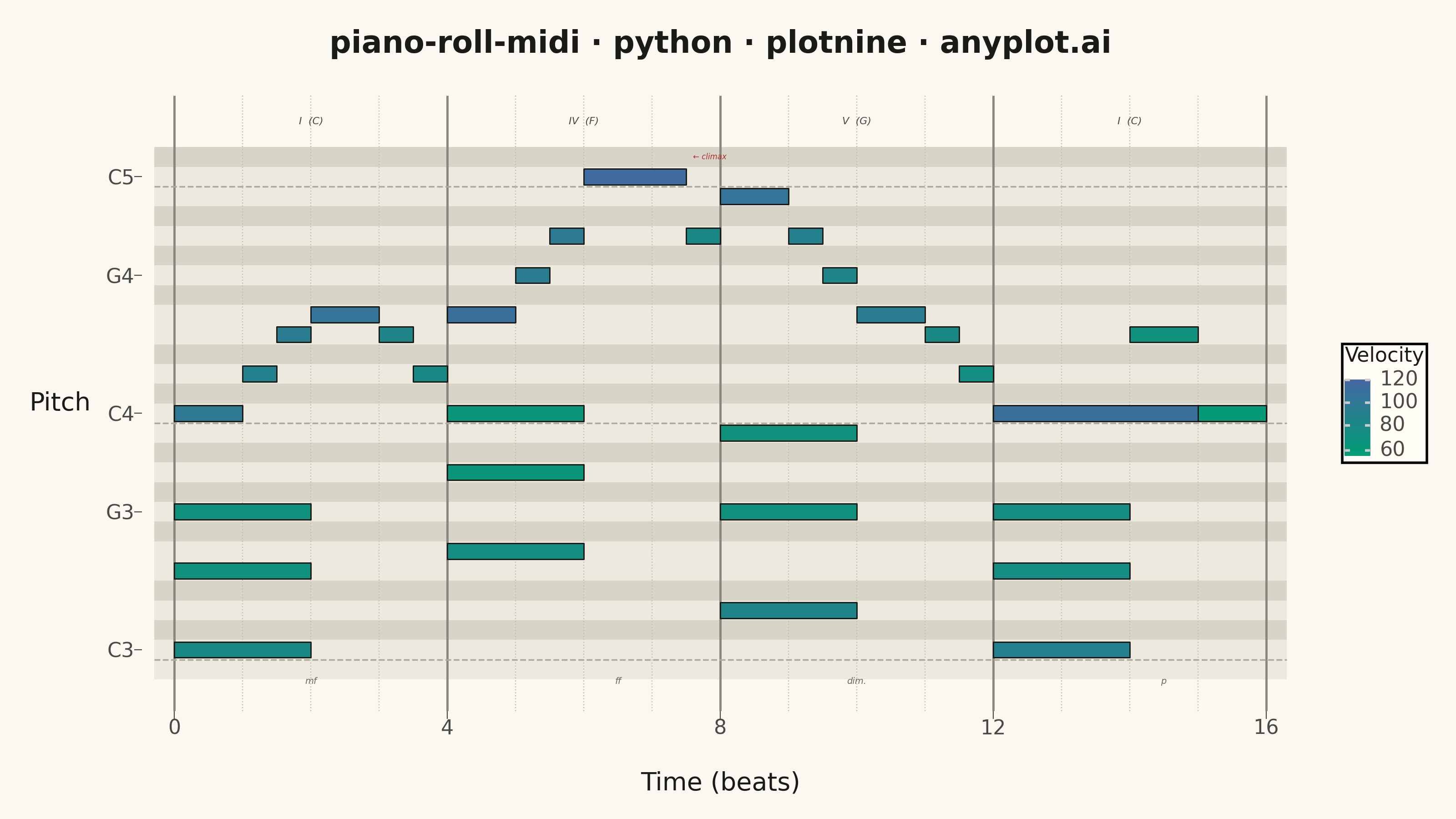
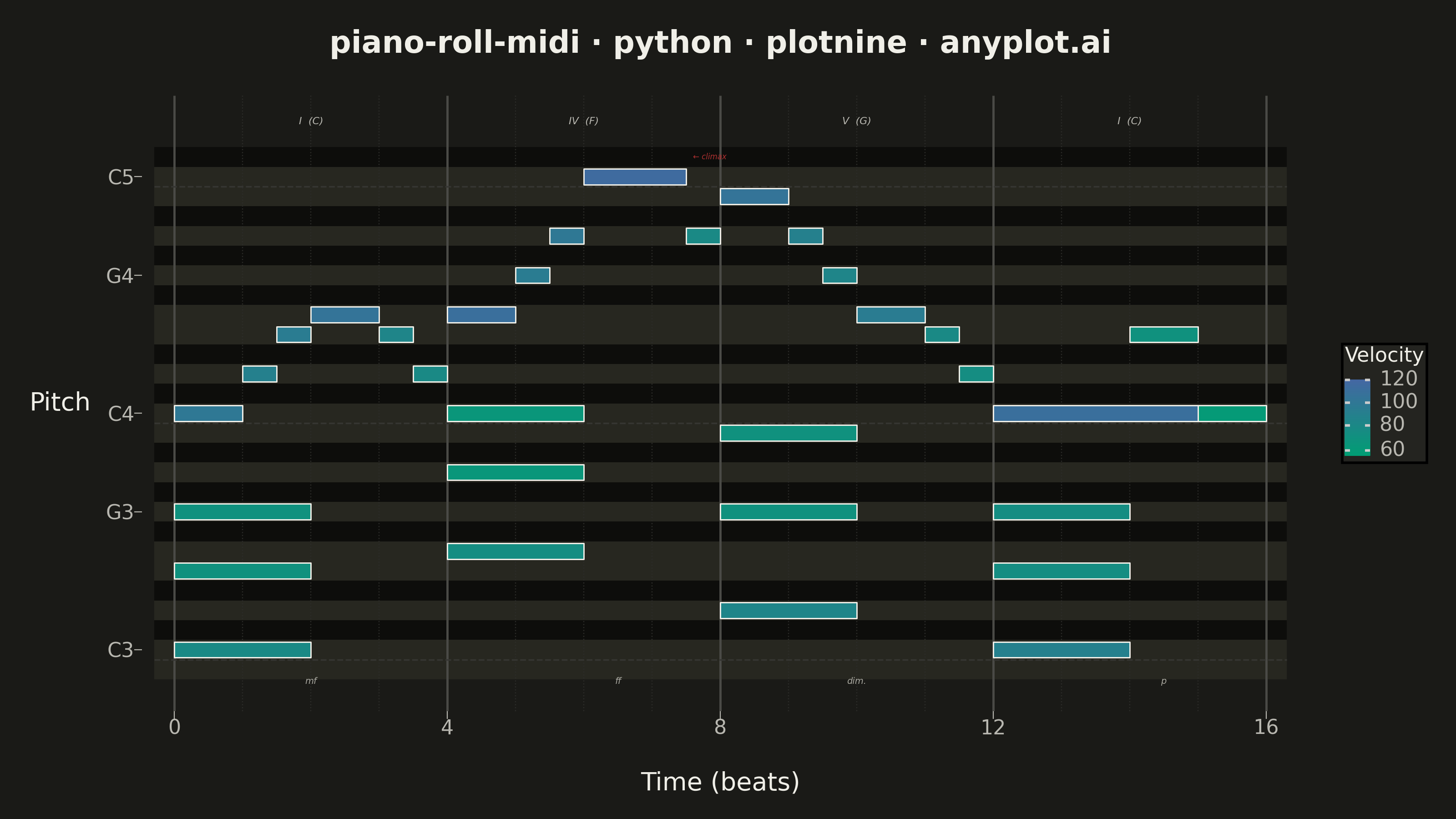
A grid-based visualization of musical notes over time, as seen in digital audio workstations (DAWs). Each note is represented as a horizontal rectangle positioned by pitch (y-axis) and time (x-axis), with bar length indicating note duration and color indicating velocity (dynamics). The background alternates between white and dark rows to mirror piano keyboard layout, with vertical grid lines marking beats and measures.
""" anyplot.ai
piano-roll-midi: MIDI Piano Roll Visualization
Library: plotnine 0.15.5 | Python 3.13.13
Quality: 91/100 | Updated: 2026-06-03
"""

import os

import numpy as np
import pandas as pd
from plotnine import (
    aes,
    annotate,
    coord_cartesian,
    element_line,
    element_rect,
    element_text,
    geom_rect,
    geom_segment,
    geom_text,
    geom_vline,
    ggplot,
    guide_colorbar,
    labs,
    scale_fill_gradient,
    scale_x_continuous,
    scale_y_continuous,
    theme,
    theme_void,
)


# Theme tokens (Imprint palette, theme-adaptive chrome)
THEME = os.getenv("ANYPLOT_THEME", "light")
PAGE_BG = "#FAF8F1" if THEME == "light" else "#1A1A17"
ELEVATED_BG = "#FFFDF6" if THEME == "light" else "#242420"
INK = "#1A1A17" if THEME == "light" else "#F0EFE8"
INK_SOFT = "#4A4A44" if THEME == "light" else "#B8B7B0"
INK_MUTED = "#6B6A63" if THEME == "light" else "#A8A79F"

# Piano key shading (theme-adaptive) — dark values boosted for visible contrast over #1A1A17
WHITE_KEY_BG = "#EDE9DE" if THEME == "light" else "#272720"
BLACK_KEY_BG = "#D8D4C8" if THEME == "light" else "#0D0D0B"
BEAT_LINE = "#C4C0B4" if THEME == "light" else "#2C2C29"
MEASURE_LINE = "#8A8780" if THEME == "light" else "#4A4A46"
OCTAVE_LINE = "#ABA89C" if THEME == "light" else "#363632"

# Data — C major → F major → G major → C major chord progression with melody
np.random.seed(42)

notes = [
    # Measure 1: C major chord + melody (mf)
    (0.0, 2.0, 48, 80),  # C3 bass
    (0.0, 2.0, 52, 70),  # E3
    (0.0, 2.0, 55, 70),  # G3
    (0.0, 1.0, 60, 100),  # C4 melody
    (1.0, 0.5, 62, 90),  # D4
    (1.5, 0.5, 64, 95),  # E4
    (2.0, 1.0, 65, 105),  # F4
    (3.0, 0.5, 64, 85),  # E4
    (3.5, 0.5, 62, 80),  # D4
    # Measure 2: F major chord + melody (f to ff)
    (4.0, 2.0, 53, 75),  # F3 bass
    (4.0, 2.0, 57, 65),  # A3
    (4.0, 2.0, 60, 65),  # C4
    (4.0, 1.0, 65, 110),  # F4 melody
    (5.0, 0.5, 67, 95),  # G4
    (5.5, 0.5, 69, 100),  # A4
    (6.0, 1.5, 72, 115),  # C5 — CLIMAX
    (7.5, 0.5, 69, 80),  # A4
    # Measure 3: G major chord + descending melody (diminuendo)
    (8.0, 2.0, 50, 85),  # D3 bass (G/D inversion)
    (8.0, 2.0, 55, 70),  # G3
    (8.0, 2.0, 59, 70),  # B3
    (8.0, 1.0, 71, 105),  # B4 melody
    (9.0, 0.5, 69, 90),  # A4
    (9.5, 0.5, 67, 85),  # G4
    (10.0, 1.0, 65, 95),  # F4
    (11.0, 0.5, 64, 80),  # E4
    (11.5, 0.5, 62, 75),  # D4
    # Measure 4: C major resolution (p, fading)
    (12.0, 2.0, 48, 90),  # C3 bass
    (12.0, 2.0, 52, 75),  # E3
    (12.0, 2.0, 55, 75),  # G3
    (12.0, 3.0, 60, 110),  # C4 — long resolution
    (14.0, 1.0, 64, 70),  # E4
    (15.0, 1.0, 60, 60),  # C4 — soft fade
]

df = pd.DataFrame(notes, columns=["start", "duration", "pitch", "velocity"])
df["end"] = df["start"] + df["duration"]
df["ymin"] = df["pitch"] - 0.4
df["ymax"] = df["pitch"] + 0.4

note_names = ["C", "C♯", "D", "D♯", "E", "F", "F♯", "G", "G♯", "A", "A♯", "B"]

pitch_min = int(df["pitch"].min()) - 1  # 47
pitch_max = int(df["pitch"].max()) + 1  # 73

# Background rows — theme-adaptive black/white key shading
black_key_semitones = {1, 3, 6, 8, 10}
bg_rows = [
    {"ymin": p - 0.5, "ymax": p + 0.5, "fill_color": BLACK_KEY_BG if p % 12 in black_key_semitones else WHITE_KEY_BG}
    for p in range(pitch_min, pitch_max + 1)
]
bg_df = pd.DataFrame(bg_rows)

# Y-axis: C (octave markers) and G (dominant) only — avoids adjacent-label crowding
label_pitches = sorted(p for p in range(pitch_min, pitch_max + 1) if p % 12 in {0, 7})
label_names = [f"{note_names[p % 12]}{p // 12 - 1}" for p in label_pitches]

# Measure structure
total_beats = 16
measure_lines = [0, 4, 8, 12, 16]
beat_lines = [b for b in range(total_beats + 1) if b not in measure_lines]

# Chord labels at measure tops
measure_labels = pd.DataFrame(
    {"x": [2, 6, 10, 14], "label": ["I  (C)", "IV  (F)", "V  (G)", "I  (C)"], "y": [pitch_max + 1.8] * 4}
)

# Dynamic markings below piano roll
dynamic_labels = pd.DataFrame({"x": [2, 6.5, 10, 14.5], "label": ["mf", "ff", "dim.", "p"], "y": [pitch_min - 0.6] * 4})

# Octave boundary lines at each C note
octave_cs = [p for p in range(pitch_min, pitch_max + 1) if p % 12 == 0]
octave_lines = pd.DataFrame(
    {"y": [c - 0.5 for c in octave_cs], "xstart": [-0.3] * len(octave_cs), "xend": [total_beats + 0.3] * len(octave_cs)}
)

title = "piano-roll-midi · python · plotnine · anyplot.ai"

# Plot
plot = (
    ggplot()
    # Background rows — black/white key distinction
    + geom_rect(
        bg_df,
        aes(xmin=-0.3, xmax=total_beats + 0.3, ymin="ymin", ymax="ymax"),
        fill=bg_df["fill_color"].tolist(),
        color=None,
        show_legend=False,
    )
    # Beat grid (subtle dotted)
    + geom_vline(xintercept=beat_lines, color=BEAT_LINE, size=0.25, linetype="dotted")
    # Measure boundaries (solid)
    + geom_vline(xintercept=measure_lines, color=MEASURE_LINE, size=0.5, linetype="solid")
    # Octave boundary lines (dashed)
    + geom_segment(
        octave_lines, aes(x="xstart", xend="xend", y="y", yend="y"), color=OCTAVE_LINE, size=0.35, linetype="dashed"
    )
    # Note rectangles — Imprint sequential colormap (green=soft → blue=loud)
    + geom_rect(df, aes(xmin="start", xmax="end", ymin="ymin", ymax="ymax", fill="velocity"), color=INK, size=0.3)
    # Climax annotation
    + annotate("text", x=7.6, y=72 + 1.0, label="← climax", size=3.0, color="#AE3030", fontstyle="italic", ha="left")
    # Chord labels at top of each measure
    + geom_text(measure_labels, aes(x="x", y="y", label="label"), size=4.0, color=INK_SOFT, fontstyle="italic")
    # Dynamic markings below
    + geom_text(dynamic_labels, aes(x="x", y="y", label="label"), size=3.5, color=INK_MUTED, fontstyle="italic")
    # Imprint sequential cmap: #009E73 (soft/piano) → #4467A3 (loud/forte)
    + scale_fill_gradient(
        low="#009E73", high="#4467A3", limits=(55, 120), name="Velocity", guide=guide_colorbar(nbin=200)
    )
    + scale_y_continuous(breaks=label_pitches, labels=label_names, expand=(0.02, 0.02))
    + scale_x_continuous(breaks=measure_lines, labels=["0", "4", "8", "12", "16"], expand=(0.01, 0.01))
    + coord_cartesian(xlim=(-0.3, total_beats + 0.3), ylim=(pitch_min - 1.5, pitch_max + 2.5))
    + labs(x="Time (beats)", y="Pitch", title=title)
    + theme_void()
    + theme(
        figure_size=(8, 4.5),
        plot_title=element_text(size=12, weight="bold", color=INK, margin={"b": 8}),
        axis_title_x=element_text(size=10, color=INK, margin={"t": 6}),
        axis_title_y=element_text(size=10, color=INK, margin={"r": 6}),
        axis_text_x=element_text(size=8, color=INK_SOFT),
        axis_text_y=element_text(size=8, color=INK_SOFT),
        axis_ticks_major=element_line(color=INK_SOFT, size=0.4),
        axis_ticks_length=3,
        legend_position="right",
        legend_title=element_text(size=8, color=INK),
        legend_text=element_text(size=8, color=INK_SOFT),
        legend_background=element_rect(fill=ELEVATED_BG, color=None),
        legend_key_height=30,
        legend_key_width=10,
        panel_background=element_rect(fill=PAGE_BG, color=None),
        plot_background=element_rect(fill=PAGE_BG, color=None),
        plot_margin=0.02,
    )
)

# Save
plot.save(f"plot-{THEME}.png", dpi=400, width=8, height=4.5, units="in", verbose=False)
Runnable source as JSON, for any HTTP client: https://api.anyplot.ai/specs/piano-roll-midi/plotnine/code. Any spec id and library id listed in llms-full.txt fit the same URL shape; every URL below is complete and callable.
{
  "spec_id": "piano-roll-midi",
  "language": "python",
  "library": "plotnine",
  "page": "https://anyplot.ai/piano-roll-midi/python/plotnine",
  "hub": "https://anyplot.ai/piano-roll-midi",
  "code_json": "https://api.anyplot.ai/specs/piano-roll-midi/plotnine/code",
  "spec_json": "https://api.anyplot.ai/specs/piano-roll-midi",
  "render_light_png": "https://storage.googleapis.com/anyplot-images/plots/piano-roll-midi/python/plotnine/plot-light.png",
  "render_dark_png": "https://storage.googleapis.com/anyplot-images/plots/piano-roll-midi/python/plotnine/plot-dark.png",
  "quality_score": 91.0,
  "license": "MIT",
  "guide": "https://anyplot.ai/llms.txt"
}
Part of MIDI Piano Roll Visualization on anyplot.ai.