The same plot in 14 other libraries — Python: Altair, Bokeh, lets-plot, Matplotlib, Plotly, plotnine, Pygal, Seaborn; Julia: Makie.jl; JavaScript: Chart.js, D3.js, Apache ECharts, Highcharts, MUI X Charts. Compare all 15 side by side: MIDI Piano Roll Visualization in Python, R, Julia and JavaScript.
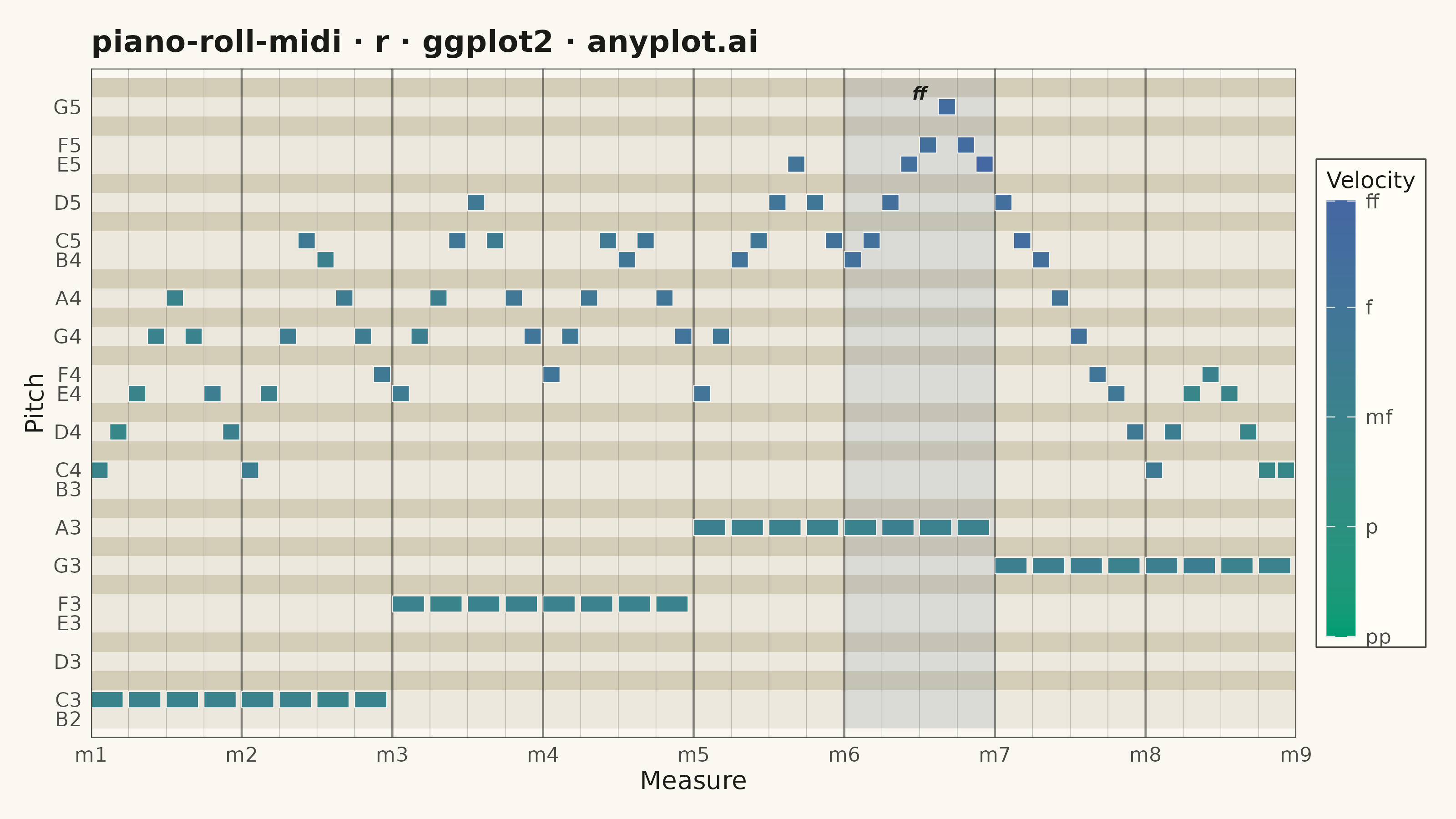
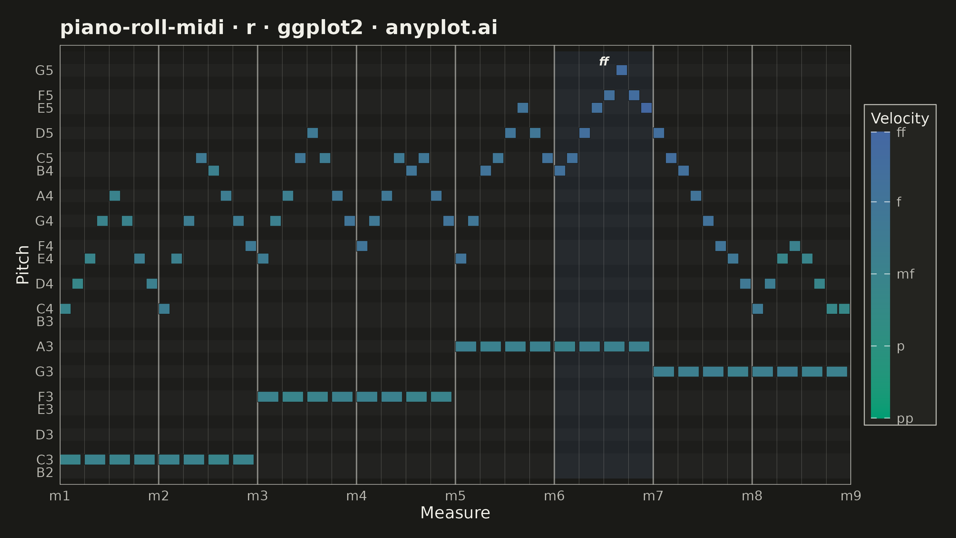
A grid-based visualization of musical notes over time, as seen in digital audio workstations (DAWs). Each note is represented as a horizontal rectangle positioned by pitch (y-axis) and time (x-axis), with bar length indicating note duration and color indicating velocity (dynamics). The background alternates between white and dark rows to mirror piano keyboard layout, with vertical grid lines marking beats and measures.
#' anyplot.ai
#' piano-roll-midi: MIDI Piano Roll Visualization
#' Library: ggplot2 3.5.1 | R 4.4.1
#' Quality: 89/100 | Created: 2026-06-03

library(ggplot2)
library(ragg)

set.seed(42)

# Theme tokens (Imprint palette)
THEME       <- Sys.getenv("ANYPLOT_THEME", "light")
PAGE_BG     <- if (THEME == "light") "#FAF8F1" else "#1A1A17"
ELEVATED_BG <- if (THEME == "light") "#FFFDF6" else "#242420"
INK         <- if (THEME == "light") "#1A1A17" else "#F0EFE8"
INK_SOFT    <- if (THEME == "light") "#4A4A44" else "#B8B7B0"

# Imprint sequential colormap for velocity: green (quiet) -> blue (loud)
CMAP_LOW  <- "#009E73"
CMAP_HIGH <- "#4467A3"

# Piano keyboard row background colors
KEY_WHITE <- if (THEME == "light") "#EBE7DC" else "#222220"
KEY_BLACK <- if (THEME == "light") "#D3CDB8" else "#1D1D1B"

NOTE_NAMES <- c("C", "C#", "D", "D#", "E", "F", "F#", "G", "G#", "A", "A#", "B")
BLACK_KEYS <- c(1L, 3L, 6L, 8L, 10L)

# --- Data: 8-measure C-major piano piece (32 beats, 4/4 time) ---------------

# Right hand: eighth notes (0.5 beat each), melodic lines building to climax
rh_pitches <- c(
  60, 62, 64, 67, 69, 67, 64, 62,   # m1: gentle ascent/descent
  60, 64, 67, 72, 71, 69, 67, 65,   # m2: arpeggiated C chord
  64, 67, 69, 72, 74, 72, 69, 67,   # m3: E-based run
  65, 67, 69, 72, 71, 72, 69, 67,   # m4: F-based figure
  64, 67, 71, 72, 74, 76, 74, 72,   # m5: climbing higher
  71, 72, 74, 76, 77, 79, 77, 76,   # m6: climax in upper register
  74, 72, 71, 69, 67, 65, 64, 62,   # m7: long descent
  60, 62, 64, 65, 64, 62, 60, 60    # m8: quiet resolution to C4
)
rh_starts    <- seq(0, 31.5, by = 0.5)
rh_durations <- rep(0.45, 64L)

# Velocity arc: mf start -> ff climax (m6) -> p resolution
vel_raw <- c(
  seq(55,  70, length.out = 8L),
  seq(68,  82, length.out = 8L),
  seq(80,  90, length.out = 8L),
  seq(88,  95, length.out = 8L),
  seq(93, 103, length.out = 8L),
  seq(103, 118, length.out = 8L),
  seq(112,  85, length.out = 8L),
  seq(80,   48, length.out = 8L)
)
rh_vel <- pmin(pmax(round(vel_raw + rnorm(64L, 0, 4)), 30L), 127L)

# Left hand: bass root on every quarter beat (C-F-Am-G progression, 2 measures each)
bass_pitches <- rep(c(48L, 53L, 57L, 55L), each = 8L)
bass_starts  <- 0:31
bass_dur     <- rep(0.85, 32L)
bass_vel     <- pmin(pmax(round(seq(62, 72, length.out = 32L) + rnorm(32L, 0, 3)), 30L), 100L)

notes_df <- data.frame(
  start    = c(rh_starts, as.numeric(bass_starts)),
  end      = c(rh_starts + rh_durations, bass_starts + bass_dur),
  pitch    = c(rh_pitches, bass_pitches),
  velocity = c(rh_vel, bass_vel)
)

# Pitch range with 1-semitone margin
pitch_min  <- min(notes_df$pitch) - 1L
pitch_max  <- max(notes_df$pitch) + 1L
all_pitches <- seq(pitch_min, pitch_max)

# Separate background row data by key type
white_rows <- all_pitches[!(all_pitches %% 12 %in% BLACK_KEYS)]
black_rows <- all_pitches[  all_pitches %% 12 %in% BLACK_KEYS]

bg_white <- data.frame(xmin = 0, xmax = 32, ymin = white_rows - 0.5, ymax = white_rows + 0.5)
bg_black <- data.frame(xmin = 0, xmax = 32, ymin = black_rows - 0.5, ymax = black_rows + 0.5)

# Y-axis: label only white keys
y_labels <- paste0(NOTE_NAMES[(white_rows %% 12) + 1], floor(white_rows / 12) - 1)

# Beat / measure grid positions (beat lines exclude measure boundaries)
beat_xs    <- (1:31)[!(1:31 %% 4 == 0)]
measure_xs <- seq(0L, 32L, by = 4L)

# Climax highlight: measure 6 (beats 20-24) is the dynamic peak (ff)
climax_df <- data.frame(xmin = 20, xmax = 24, ymin = pitch_min - 0.5, ymax = pitch_max + 0.5)

plot_title <- "piano-roll-midi · r · ggplot2 · anyplot.ai"

# --- Plot -------------------------------------------------------------------
p <- ggplot() +
  # Piano keyboard background: white keys
  geom_rect(
    data = bg_white,
    aes(xmin = xmin, xmax = xmax, ymin = ymin, ymax = ymax),
    fill = KEY_WHITE, color = NA
  ) +
  # Piano keyboard background: black keys
  geom_rect(
    data = bg_black,
    aes(xmin = xmin, xmax = xmax, ymin = ymin, ymax = ymax),
    fill = KEY_BLACK, color = NA
  ) +
  # Subtle translucent highlight at dynamic climax (m6, beats 20-24)
  geom_rect(
    data = climax_df,
    aes(xmin = xmin, xmax = xmax, ymin = ymin, ymax = ymax),
    fill = CMAP_HIGH, color = NA, alpha = 0.10
  ) +
  # Beat subdivision lines (very faint)
  geom_vline(
    xintercept = beat_xs,
    color = INK_SOFT, linewidth = 0.12, alpha = 0.35
  ) +
  # Measure boundary lines (stronger)
  geom_vline(
    xintercept = measure_xs,
    color = INK, linewidth = 0.4, alpha = 0.5
  ) +
  # MIDI notes colored by velocity
  geom_rect(
    data = notes_df,
    aes(
      xmin = start, xmax = end,
      ymin = pitch - 0.42, ymax = pitch + 0.42,
      fill = velocity
    ),
    color = PAGE_BG, linewidth = 0.15
  ) +
  # "ff" annotation marking the dynamic peak
  annotate(
    "text", x = 22, y = pitch_max - 0.3,
    label = "ff", color = INK, size = 2.5, fontface = "bold.italic"
  ) +
  # Imprint sequential colormap for velocity (green=quiet, blue=loud)
  scale_fill_gradient(
    low    = CMAP_LOW,
    high   = CMAP_HIGH,
    limits = c(0, 127),
    name   = "Velocity",
    breaks = c(0, 32, 64, 96, 127),
    labels = c("pp", "p", "mf", "f", "ff")
  ) +
  scale_x_continuous(
    name   = "Measure",
    breaks = seq(0, 32, by = 4),
    labels = paste0("m", 1:9),
    expand = expansion(add = c(0, 0))
  ) +
  scale_y_continuous(
    name   = "Pitch",
    breaks = white_rows,
    labels = y_labels,
    expand = expansion(add = c(0.5, 0.5))
  ) +
  labs(title = plot_title) +
  theme_minimal(base_size = 8) +
  theme(
    plot.background   = element_rect(fill = PAGE_BG, color = PAGE_BG),
    panel.background  = element_rect(fill = PAGE_BG, color = NA),
    panel.grid.major  = element_blank(),
    panel.grid.minor  = element_blank(),
    panel.border      = element_rect(color = INK_SOFT, fill = NA, linewidth = 0.35),
    axis.title        = element_text(color = INK,      size = 10),
    axis.text         = element_text(color = INK_SOFT, size = 8),
    axis.text.y       = element_text(color = INK_SOFT, size = 8),
    plot.title        = element_text(color = INK,      size = 12, face = "bold"),
    legend.background = element_rect(fill = ELEVATED_BG, color = INK_SOFT, linewidth = 0.3),
    legend.text       = element_text(color = INK_SOFT, size = 8),
    legend.title      = element_text(color = INK,      size = 9),
    legend.position   = "right",
    plot.margin       = margin(12, 12, 10, 10)
  ) +
  guides(
    fill = guide_colorbar(
      barheight = 12,
      barwidth  = 0.8
    )
  )

# --- Save -------------------------------------------------------------------
ggsave(
  filename = sprintf("plot-%s.png", THEME),
  plot     = p,
  device   = ragg::agg_png,
  width    = 8,
  height   = 4.5,
  units    = "in",
  dpi      = 400
)
Runnable source as JSON, for any HTTP client: https://api.anyplot.ai/specs/piano-roll-midi/ggplot2/code. Any spec id and library id listed in llms-full.txt fit the same URL shape; every URL below is complete and callable.
{
  "spec_id": "piano-roll-midi",
  "language": "r",
  "library": "ggplot2",
  "page": "https://anyplot.ai/piano-roll-midi/r/ggplot2",
  "hub": "https://anyplot.ai/piano-roll-midi",
  "code_json": "https://api.anyplot.ai/specs/piano-roll-midi/ggplot2/code",
  "spec_json": "https://api.anyplot.ai/specs/piano-roll-midi",
  "render_light_png": "https://storage.googleapis.com/anyplot-images/plots/piano-roll-midi/r/ggplot2/plot-light.png",
  "render_dark_png": "https://storage.googleapis.com/anyplot-images/plots/piano-roll-midi/r/ggplot2/plot-dark.png",
  "quality_score": 89.0,
  "license": "MIT",
  "guide": "https://anyplot.ai/llms.txt"
}
Part of MIDI Piano Roll Visualization on anyplot.ai.