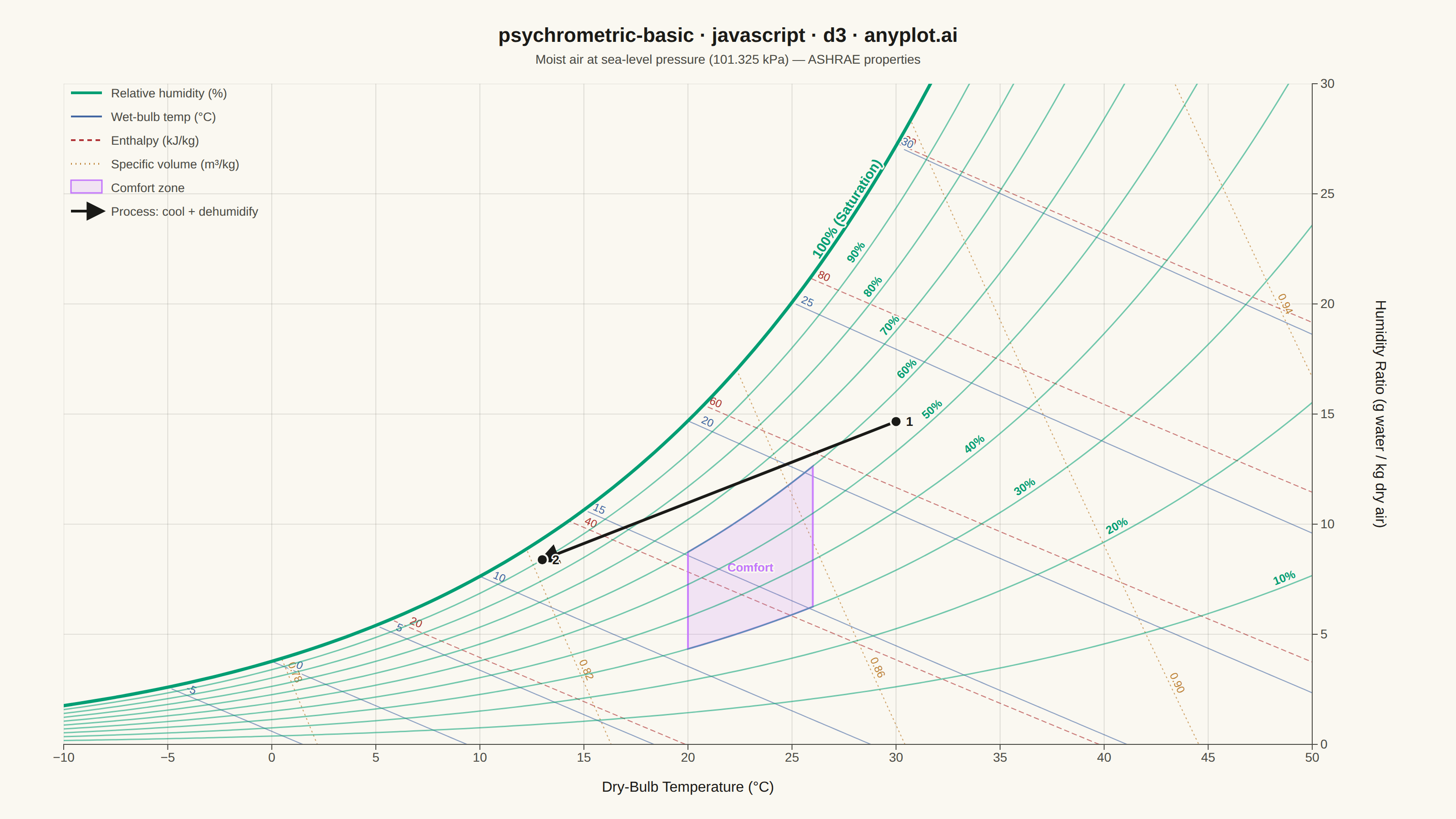
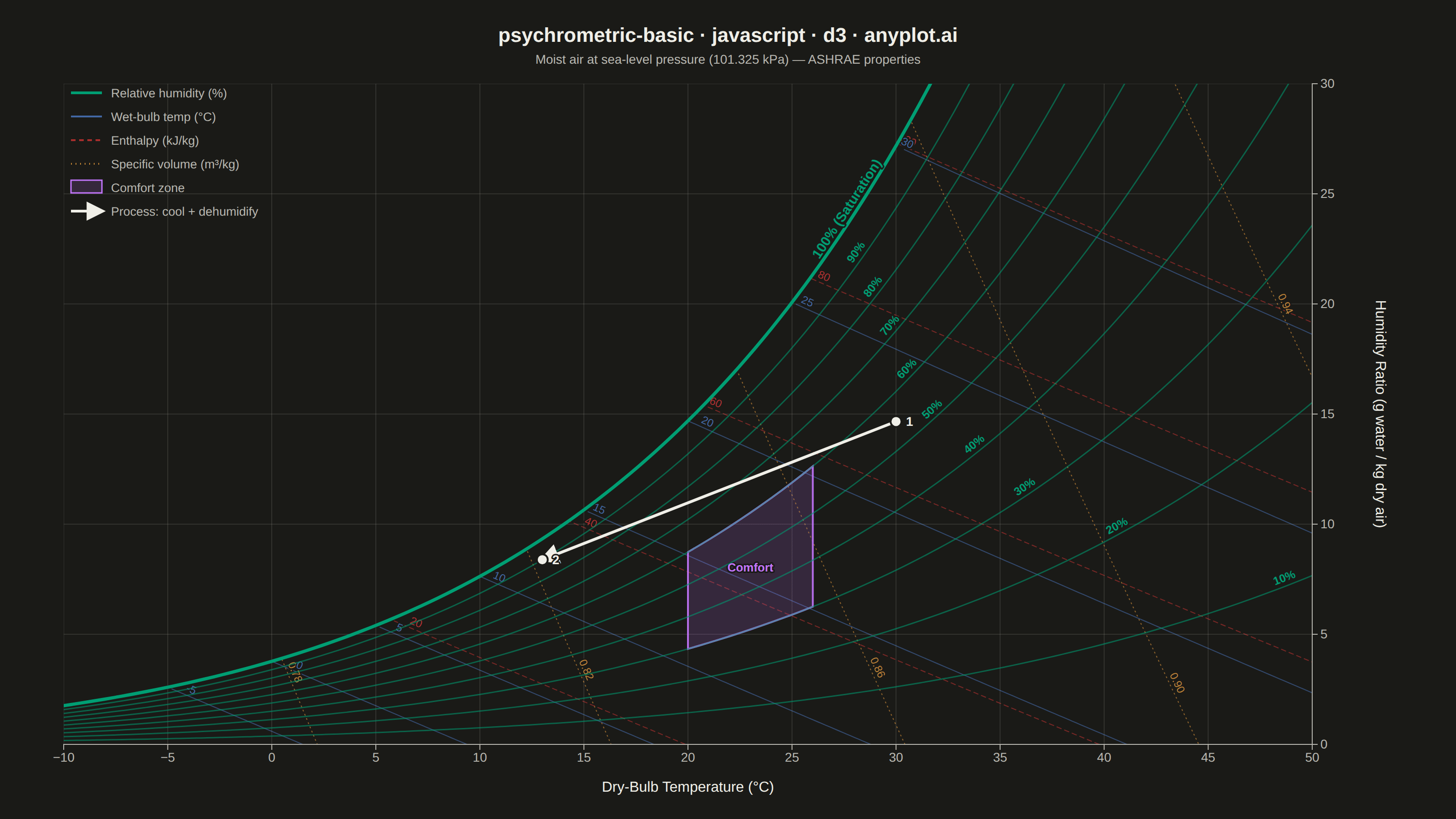
A psychrometric chart plots dry-bulb temperature against humidity ratio, overlaid with curves for relative humidity, wet-bulb temperature, enthalpy, and specific volume. It is the fundamental tool for HVAC system design and air conditioning process analysis. The chart reveals the thermodynamic properties of moist air at a glance, enabling engineers to trace heating, cooling, humidification, and dehumidification processes as paths on the diagram.
// anyplot.ai
// psychrometric-basic: Psychrometric Chart for HVAC
// Library: d3 7.9.0 | JavaScript 22.22.3
// Quality: 92/100 | Created: 2026-06-16
//# anyplot-orientation: landscape
// anyplot.ai
// psychrometric-basic: Psychrometric Chart for HVAC
// Library: d3 7.9.0 | JavaScript 22
// Quality: pending | Created: 2026-06-16

const t = window.ANYPLOT_TOKENS;
const { width, height } = window.ANYPLOT_SIZE;

// ── Moist-air psychrometrics at sea-level pressure (ASHRAE, 101.325 kPa) ──────
// All thermodynamic property lines are derived analytically from these
// closed-form relations — nothing is loaded from disk or the network.
const P = 101.325; // total atmospheric pressure, kPa

// Saturation vapour pressure over water (kPa), Tetens approximation, T in °C
const pws = (T) => 0.61078 * Math.exp((17.27 * T) / (T + 237.3));

// Humidity ratio (g water / kg dry air) from a vapour pressure (kPa)
const wFromPw = (pw) => (621.945 * pw) / (P - pw);

// W along a constant relative-humidity curve (rh as a fraction 0–1)
const wFromRH = (T, rh) => wFromPw(rh * pws(T));

// Saturation humidity ratio (100 % RH)
const wSat = (T) => wFromPw(pws(T));

// W along a constant wet-bulb line (ASHRAE psychrometric energy balance)
const wFromWetBulb = (Tdb, Twb) => {
  const wsWb = wSat(Twb) / 1000; // kg/kg at saturation, evaluated at T_wb
  const w =
    ((2501 - 2.326 * Twb) * wsWb - 1.006 * (Tdb - Twb)) /
    (2501 + 1.86 * Tdb - 4.186 * Twb);
  return w * 1000;
};

// W along a constant-enthalpy line, h in kJ/kg dry air
const wFromEnthalpy = (T, h) => ((h - 1.006 * T) / (2501 + 1.86 * T)) * 1000;

// W along a constant specific-volume line, v in m³/kg dry air
const wFromVolume = (T, v) =>
  (((v * P) / (0.287042 * (T + 273.15)) - 1) / 1.607858) * 1000;

// ── Domain ───────────────────────────────────────────────────────────────────
const T_MIN = -10;
const T_MAX = 50;
const W_MIN = 0;
const W_MAX = 30; // g/kg — caps the chart; the saturation curve exits the top

// Property-line families to draw
const rhValues = [10, 20, 30, 40, 50, 60, 70, 80, 90, 100];
const wetBulbValues = [-5, 0, 5, 10, 15, 20, 25, 30];
const enthalpyValues = [20, 40, 60, 80, 100];
const volumeValues = [0.78, 0.82, 0.86, 0.9, 0.94];

// ── Theme-mapped Imprint colours ─────────────────────────────────────────────
const RH_COLOR = t.palette[0]; // brand green — primary family
const WB_COLOR = t.palette[2]; // blue   — wet-bulb (evaporative cooling / water)
const ENTH_COLOR = t.palette[4]; // red    — enthalpy (energy / heat)
const VOL_COLOR = t.palette[3]; // ochre  — specific volume
const COMFORT_COLOR = t.palette[1]; // lavender — comfort zone
const PROCESS_COLOR = t.ink; // neutral ink — HVAC process path

// ── Layout ───────────────────────────────────────────────────────────────────
const margin = { top: 92, right: 158, bottom: 82, left: 70 };
const iw = width - margin.left - margin.right;
const ih = height - margin.top - margin.bottom;

const x = d3.scaleLinear().domain([T_MIN, T_MAX]).range([0, iw]);
const y = d3.scaleLinear().domain([W_MIN, W_MAX]).range([ih, 0]);

const svg = d3
  .select("#container")
  .append("svg")
  .attr("width", width)
  .attr("height", height);

// Clip so property lines that leave the saturation envelope are trimmed cleanly
const defs = svg.append("defs");
defs
  .append("clipPath")
  .attr("id", "plotClip")
  .append("rect")
  .attr("width", iw)
  .attr("height", ih);

defs
  .append("marker")
  .attr("id", "processArrow")
  .attr("viewBox", "0 0 10 10")
  .attr("refX", 8)
  .attr("refY", 5)
  .attr("markerWidth", 7)
  .attr("markerHeight", 7)
  .attr("orient", "auto-start-reverse")
  .append("path")
  .attr("d", "M0,0 L10,5 L0,10 Z")
  .attr("fill", PROCESS_COLOR);

// The moist-air region lives below the saturation curve; wet-bulb, enthalpy and
// specific-volume lines are only physical there, so clip them to it.
const satClipPts = [[x(T_MIN), ih]];
for (let T = T_MIN; T <= T_MAX + 1e-9; T += 0.4) {
  satClipPts.push([x(T), y(Math.min(wSat(T), W_MAX))]);
}
satClipPts.push([x(T_MAX), ih]);
defs
  .append("clipPath")
  .attr("id", "satClip")
  .append("path")
  .attr("d", "M" + satClipPts.map((p) => p.join(",")).join("L") + "Z");

const g = svg
  .append("g")
  .attr("transform", `translate(${margin.left},${margin.top})`);
const plot = g.append("g").attr("clip-path", "url(#plotClip)");
const moist = plot.append("g").attr("clip-path", "url(#satClip)");

// ── Reference grid (subtle) ──────────────────────────────────────────────────
const xTicks = d3.range(T_MIN, T_MAX + 1, 5);
const yTicks = d3.range(W_MIN, W_MAX + 1, 5);
plot
  .append("g")
  .selectAll("line")
  .data(xTicks)
  .join("line")
  .attr("x1", (d) => x(d))
  .attr("x2", (d) => x(d))
  .attr("y1", 0)
  .attr("y2", ih)
  .attr("stroke", t.grid)
  .attr("stroke-width", 0.8);
plot
  .append("g")
  .selectAll("line")
  .data(yTicks)
  .join("line")
  .attr("x1", 0)
  .attr("x2", iw)
  .attr("y1", (d) => y(d))
  .attr("y2", (d) => y(d))
  .attr("stroke", t.grid)
  .attr("stroke-width", 0.8);

// ── Sampling + curve helpers ─────────────────────────────────────────────────
const sample = (fn, step = 0.4) => {
  const pts = [];
  for (let T = T_MIN; T <= T_MAX + 1e-9; T += step) {
    const W = fn(T);
    if (Number.isFinite(W)) pts.push({ T, W });
  }
  return pts;
};

const lineGen = d3
  .line()
  .x((d) => x(d.T))
  .y((d) => y(d.W))
  .curve(d3.curveMonotoneX);

const drawCurve = (pts, color, width, dash, opacity, group = plot) =>
  group
    .append("path")
    .datum(pts)
    .attr("d", lineGen)
    .attr("fill", "none")
    .attr("stroke", color)
    .attr("stroke-width", width)
    .attr("stroke-dasharray", dash)
    .attr("stroke-opacity", opacity)
    .attr("stroke-linecap", "round");

// In-bounds sample point whose W sits closest to a target — used to anchor
// labels. `belowSat` keeps anchors inside the moist-air region (below 100 % RH).
const anchorAtW = (pts, targetW, pad = 1, belowSat = false) => {
  let best = null;
  let bestD = Infinity;
  for (const p of pts) {
    if (p.W < W_MIN + pad || p.W > W_MAX - pad) continue;
    if (p.T < T_MIN + pad || p.T > T_MAX - pad) continue;
    if (belowSat && p.W > wSat(p.T) - 0.6) continue;
    const d = Math.abs(p.W - targetW);
    if (d < bestD) {
      bestD = d;
      best = p;
    }
  }
  return best;
};

// Highest valid point still below saturation — anchors a diagonal family's label
// up near where the line meets the saturation curve (classic chart placement).
const anchorNearSat = (pts, pad = 1) => {
  let best = null;
  for (const p of pts) {
    if (p.W < W_MIN + pad || p.W > W_MAX - pad) continue;
    if (p.T < T_MIN + pad || p.T > T_MAX - pad) continue;
    if (p.W > wSat(p.T) - 0.6) continue;
    if (!best || p.W > best.W) best = p;
  }
  return best;
};

// Local pixel-space tangent angle (degrees) at a temperature, for rotated labels
const tangentDeg = (fn, T) => {
  const dx = x(T + 1) - x(T - 1);
  const dy = y(fn(T + 1)) - y(fn(T - 1));
  return (Math.atan2(dy, dx) * 180) / Math.PI;
};

const halo = (sel) =>
  sel
    .attr("stroke", t.pageBg)
    .attr("stroke-width", 3.2)
    .attr("paint-order", "stroke")
    .attr("stroke-linejoin", "round");

// ── Specific-volume lines (drawn first, behind everything) ───────────────────
volumeValues.forEach((v) => {
  const pts = sample((T) => wFromVolume(T, v));
  drawCurve(pts, VOL_COLOR, 1.1, "1 4", 0.7, moist);
  const a = anchorAtW(pts, 3, 1.5, true);
  if (a) {
    halo(
      plot
        .append("text")
        .attr("transform", `translate(${x(a.T)},${y(a.W)}) rotate(${tangentDeg((T) => wFromVolume(T, v), a.T)})`)
        .attr("text-anchor", "middle")
        .attr("dy", -4)
        .attr("fill", VOL_COLOR)
        .style("font-size", "12px")
        .text(v.toFixed(2)),
    );
  }
});

// ── Constant-enthalpy lines ──────────────────────────────────────────────────
enthalpyValues.forEach((h) => {
  const pts = sample((T) => wFromEnthalpy(T, h));
  drawCurve(pts, ENTH_COLOR, 1.1, "5 4", 0.62, moist);
  const a = anchorNearSat(pts, 1.5);
  if (a) {
    halo(
      plot
        .append("text")
        .attr("transform", `translate(${x(a.T)},${y(a.W)}) rotate(${tangentDeg((T) => wFromEnthalpy(T, h), a.T)})`)
        .attr("text-anchor", "middle")
        .attr("dy", -4)
        .attr("fill", ENTH_COLOR)
        .style("font-size", "12px")
        .text(h),
    );
  }
});

// ── Constant wet-bulb lines ──────────────────────────────────────────────────
wetBulbValues.forEach((twb) => {
  const pts = sample((T) => (T >= twb ? wFromWetBulb(T, twb) : NaN)).filter(
    (p) => Number.isFinite(p.W),
  );
  if (pts.length < 2) return;
  drawCurve(pts, WB_COLOR, 1.1, null, 0.6, moist);
  const a = anchorNearSat(pts, 1.5);
  if (a) {
    halo(
      plot
        .append("text")
        .attr("transform", `translate(${x(a.T)},${y(a.W)}) rotate(${tangentDeg((T) => wFromWetBulb(T, twb), a.T)})`)
        .attr("text-anchor", "middle")
        .attr("dy", -4)
        .attr("fill", WB_COLOR)
        .style("font-size", "12px")
        .text(twb),
    );
  }
});

// ── Comfort zone (≈20–26 °C, 30–60 % RH) — bounded by RH curves ──────────────
const comfortPts = [];
for (let T = 20; T <= 26.001; T += 0.5) comfortPts.push([x(T), y(wFromRH(T, 0.3))]);
for (let rh = 0.3; rh <= 0.601; rh += 0.05) comfortPts.push([x(26), y(wFromRH(26, rh))]);
for (let T = 26; T >= 19.999; T -= 0.5) comfortPts.push([x(T), y(wFromRH(T, 0.6))]);
for (let rh = 0.6; rh >= 0.299; rh -= 0.05) comfortPts.push([x(20), y(wFromRH(20, rh))]);
plot
  .append("path")
  .attr("d", "M" + comfortPts.map((p) => p.join(",")).join("L") + "Z")
  .attr("fill", COMFORT_COLOR)
  .attr("fill-opacity", 0.16)
  .attr("stroke", COMFORT_COLOR)
  .attr("stroke-width", 2)
  .attr("stroke-opacity", 0.9);
halo(
  plot
    .append("text")
    .attr("x", x(23))
    .attr("y", y(wFromRH(23, 0.45)))
    .attr("text-anchor", "middle")
    .attr("fill", COMFORT_COLOR)
    .style("font-size", "13px")
    .style("font-weight", "700")
    .text("Comfort"),
);

// ── Relative-humidity curves (10–100 %); saturation is prominent ─────────────
rhValues.forEach((rh) => {
  const frac = rh / 100;
  const pts = sample((T) => wFromRH(T, frac));
  const saturation = rh === 100;
  drawCurve(
    pts,
    RH_COLOR,
    saturation ? 3.6 : 1.5,
    null,
    saturation ? 1 : 0.55,
  );
  // RH labels ride up each curve; stagger by targeting progressively higher W
  const targetW = saturation ? 24 : Math.min(26, 6 + rh * 0.18);
  const a = anchorAtW(pts, targetW, saturation ? 2 : 1.2);
  if (a) {
    halo(
      plot
        .append("text")
        .attr("transform", `translate(${x(a.T)},${y(a.W)}) rotate(${tangentDeg((T) => wFromRH(T, frac), a.T)})`)
        .attr("text-anchor", "middle")
        .attr("dy", -5)
        .attr("fill", RH_COLOR)
        .style("font-size", saturation ? "15px" : "12.5px")
        .style("font-weight", saturation ? "700" : "600")
        .text(saturation ? "100% (Saturation)" : rh + "%"),
    );
  }
});

// ── Example HVAC process: cooling & dehumidification ─────────────────────────
const state1 = { T: 30, rh: 0.55 };
const state2 = { T: 13, rh: 0.9 };
const p1 = { x: x(state1.T), y: y(wFromRH(state1.T, state1.rh)) };
const p2 = { x: x(state2.T), y: y(wFromRH(state2.T, state2.rh)) };
plot
  .append("line")
  .attr("x1", p1.x)
  .attr("y1", p1.y)
  .attr("x2", p2.x)
  .attr("y2", p2.y)
  .attr("stroke", PROCESS_COLOR)
  .attr("stroke-width", 3.2)
  .attr("marker-end", "url(#processArrow)");
[
  { p: p1, label: "1" },
  { p: p2, label: "2" },
].forEach(({ p, label }) => {
  plot
    .append("circle")
    .attr("cx", p.x)
    .attr("cy", p.y)
    .attr("r", 6)
    .attr("fill", PROCESS_COLOR)
    .attr("stroke", t.pageBg)
    .attr("stroke-width", 2);
  halo(
    plot
      .append("text")
      .attr("x", p.x + 11)
      .attr("y", p.y + 5)
      .attr("fill", t.ink)
      .style("font-size", "14px")
      .style("font-weight", "700")
      .text(label),
  );
});

// ── Axes ─────────────────────────────────────────────────────────────────────
const axB = g
  .append("g")
  .attr("transform", `translate(0,${ih})`)
  .call(d3.axisBottom(x).tickValues(xTicks).tickSize(6).tickFormat(d3.format("d")));
axB.selectAll("text").attr("fill", t.inkSoft).style("font-size", "14px");
axB.selectAll(".tick line").attr("stroke", t.inkSoft);
axB.select(".domain").attr("stroke", t.inkSoft);

const axR = g
  .append("g")
  .attr("transform", `translate(${iw},0)`)
  .call(d3.axisRight(y).tickValues(yTicks).tickSize(6).tickFormat(d3.format("d")));
axR.selectAll("text").attr("fill", t.inkSoft).style("font-size", "14px");
axR.selectAll(".tick line").attr("stroke", t.inkSoft);
axR.select(".domain").attr("stroke", t.inkSoft);

g.append("text")
  .attr("x", iw / 2)
  .attr("y", ih + 52)
  .attr("text-anchor", "middle")
  .attr("fill", t.ink)
  .style("font-size", "16px")
  .text("Dry-Bulb Temperature (°C)");

g.append("text")
  .attr("transform", `translate(${iw + 70},${ih / 2}) rotate(90)`)
  .attr("text-anchor", "middle")
  .attr("fill", t.ink)
  .style("font-size", "16px")
  .text("Humidity Ratio (g water / kg dry air)");

// ── Legend (upper-left, in the impossible region above saturation) ───────────
const legend = g.append("g").attr("transform", `translate(8,6)`);
const legendItems = [
  { color: RH_COLOR, dash: null, w: 3, label: "Relative humidity (%)" },
  { color: WB_COLOR, dash: null, w: 2, label: "Wet-bulb temp (°C)" },
  { color: ENTH_COLOR, dash: "5 4", w: 2, label: "Enthalpy (kJ/kg)" },
  { color: VOL_COLOR, dash: "1 4", w: 2, label: "Specific volume (m³/kg)" },
  { color: COMFORT_COLOR, dash: null, w: 2, label: "Comfort zone", swatch: true },
  { color: PROCESS_COLOR, dash: null, w: 3, label: "Process: cool + dehumidify", arrow: true },
];
legendItems.forEach((it, i) => {
  const yy = i * 26 + 4;
  if (it.swatch) {
    legend
      .append("rect")
      .attr("x", 0)
      .attr("y", yy - 8)
      .attr("width", 34)
      .attr("height", 14)
      .attr("fill", it.color)
      .attr("fill-opacity", 0.16)
      .attr("stroke", it.color)
      .attr("stroke-width", 1.5);
  } else {
    legend
      .append("line")
      .attr("x1", 0)
      .attr("x2", 34)
      .attr("y1", yy)
      .attr("y2", yy)
      .attr("stroke", it.color)
      .attr("stroke-width", it.w)
      .attr("stroke-dasharray", it.dash)
      .attr("marker-end", it.arrow ? "url(#processArrow)" : null);
  }
  legend
    .append("text")
    .attr("x", 44)
    .attr("y", yy + 5)
    .attr("fill", t.inkSoft)
    .style("font-size", "13.5px")
    .text(it.label);
});

// ── Title ────────────────────────────────────────────────────────────────────
svg
  .append("text")
  .attr("x", width / 2)
  .attr("y", 46)
  .attr("text-anchor", "middle")
  .attr("fill", t.ink)
  .style("font-size", "22px")
  .style("font-weight", "600")
  .text("psychrometric-basic · javascript · d3 · anyplot.ai");

svg
  .append("text")
  .attr("x", width / 2)
  .attr("y", 70)
  .attr("text-anchor", "middle")
  .attr("fill", t.inkSoft)
  .style("font-size", "14px")
  .text("Moist air at sea-level pressure (101.325 kPa) — ASHRAE properties");
Runnable source as JSON, for any HTTP client: https://api.anyplot.ai/specs/psychrometric-basic/d3/code. Any spec id and library id listed in llms-full.txt fit the same URL shape; every URL below is complete and callable.
{
  "spec_id": "psychrometric-basic",
  "language": "javascript",
  "library": "d3",
  "page": "https://anyplot.ai/psychrometric-basic/javascript/d3",
  "hub": "https://anyplot.ai/psychrometric-basic",
  "code_json": "https://api.anyplot.ai/specs/psychrometric-basic/d3/code",
  "spec_json": "https://api.anyplot.ai/specs/psychrometric-basic",
  "render_light_png": "https://storage.googleapis.com/anyplot-images/plots/psychrometric-basic/javascript/d3/plot-light.png",
  "render_dark_png": "https://storage.googleapis.com/anyplot-images/plots/psychrometric-basic/javascript/d3/plot-dark.png",
  "interactive_light_html": "https://storage.googleapis.com/anyplot-images/plots/psychrometric-basic/javascript/d3/plot-light.html",
  "interactive_dark_html": "https://storage.googleapis.com/anyplot-images/plots/psychrometric-basic/javascript/d3/plot-dark.html",
  "quality_score": 92.0,
  "license": "MIT",
  "guide": "https://anyplot.ai/llms.txt"
}
Part of Psychrometric Chart for HVAC on anyplot.ai.