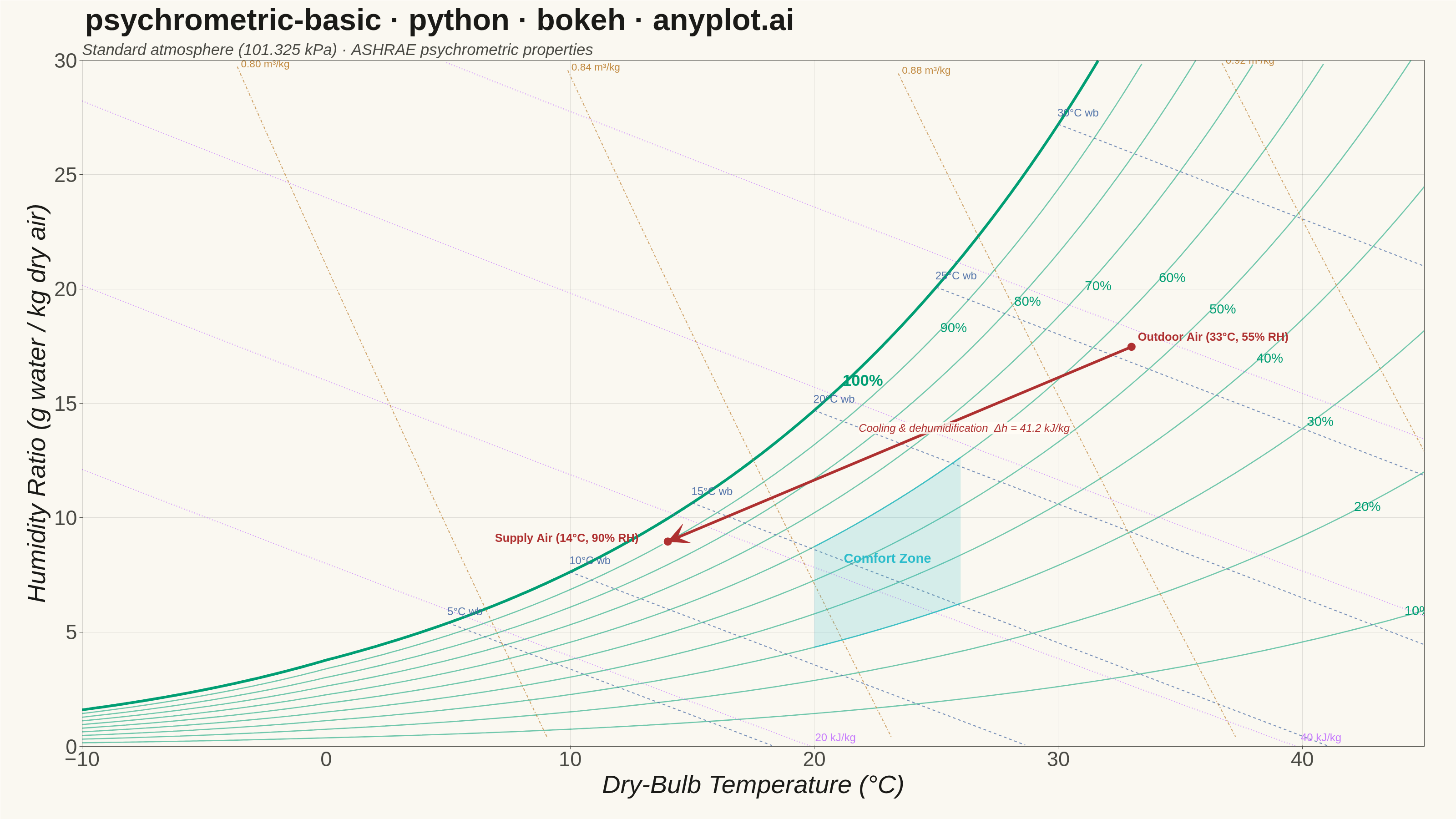
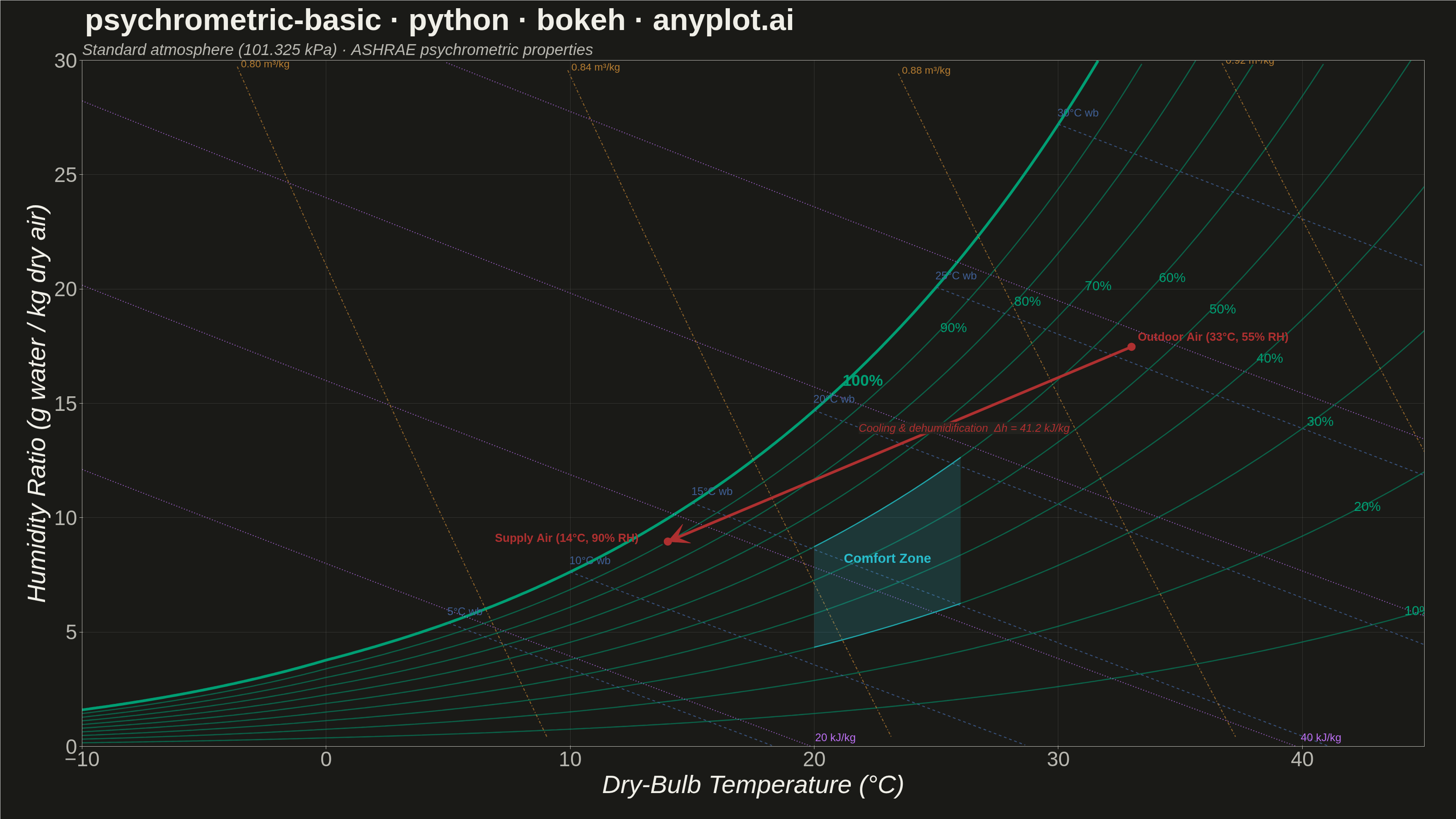
A psychrometric chart plots dry-bulb temperature against humidity ratio, overlaid with curves for relative humidity, wet-bulb temperature, enthalpy, and specific volume. It is the fundamental tool for HVAC system design and air conditioning process analysis. The chart reveals the thermodynamic properties of moist air at a glance, enabling engineers to trace heating, cooling, humidification, and dehumidification processes as paths on the diagram.
""" anyplot.ai
psychrometric-basic: Psychrometric Chart for HVAC
Library: bokeh 3.9.1 | Python 3.13.13
Quality: 92/100 | Updated: 2026-06-16
"""

import base64
import os
import time
from pathlib import Path

import numpy as np
from bokeh.io import output_file, save
from bokeh.models import Arrow, Band, ColumnDataSource, Label, Title, VeeHead
from bokeh.plotting import figure
from selenium import webdriver
from selenium.webdriver.chrome.options import Options


# Theme-adaptive chrome (see prompts/default-style-guide.md "Theme-adaptive Chrome")
THEME = os.getenv("ANYPLOT_THEME", "light")
PAGE_BG = "#FAF8F1" if THEME == "light" else "#1A1A17"
ELEVATED_BG = "#FFFDF6" if THEME == "light" else "#242420"
INK = "#1A1A17" if THEME == "light" else "#F0EFE8"
INK_SOFT = "#4A4A44" if THEME == "light" else "#B8B7B0"

# Imprint palette — each psychrometric property family gets one hue.
RH_COLOR = "#009E73"  # brand green — relative humidity (first series, always #009E73)
WB_COLOR = "#4467A3"  # blue — wet-bulb temperature (cool/temperature cue)
ENTH_COLOR = "#C475FD"  # lavender — enthalpy
SV_COLOR = "#BD8233"  # ochre — specific volume
COMFORT_COLOR = "#2ABCCD"  # cyan — comfort-zone region
PROCESS_COLOR = "#AE3030"  # matte red — highlighted HVAC process path

# Constants — standard sea-level atmosphere
P_ATM = 101325.0  # Pa
# ASHRAE saturation-pressure coefficients (over liquid water, t >= 0 °C)
C8, C9, C10, C11, C12, C13 = (-5.8002206e3, 1.3914993, -4.8640239e-2, 4.1764768e-5, -1.4452093e-8, 6.5459673)
# Over ice (t < 0 °C)
C1, C2, C3, C4, C5, C6, C7 = (
    -5.6745359e3,
    6.3925247,
    -9.677843e-3,
    6.2215701e-7,
    2.0747825e-9,
    -9.484024e-13,
    4.1635019,
)

# Data — saturation vapor pressure across the dry-bulb range
t_db = np.linspace(-10, 45, 400)
tk = t_db + 273.15
psat = np.where(
    tk >= 273.15,
    np.exp(C8 / tk + C9 + C10 * tk + C11 * tk**2 + C12 * tk**3 + C13 * np.log(tk)),
    np.exp(C1 / tk + C2 + C3 * tk + C4 * tk**2 + C5 * tk**3 + C6 * tk**4 + C7 * np.log(tk)),
)

# Plot
title = "psychrometric-basic · python · bokeh · anyplot.ai"
p = figure(
    width=3200,
    height=1800,
    title=title,
    x_axis_label="Dry-Bulb Temperature (°C)",
    y_axis_label="Humidity Ratio (g water / kg dry air)",
    toolbar_location=None,
    x_range=(-10, 45),
    y_range=(0, 30),
    min_border_bottom=160,
    min_border_left=180,
    min_border_top=130,
    min_border_right=70,
)

# --- Relative-humidity curves (10 % to 100 %) ---
rh_label_x = {10: 44, 20: 42, 30: 40, 40: 38, 50: 36, 60: 34, 70: 31, 80: 28, 90: 25, 100: 21}
for rh_pct in range(10, 101, 10):
    pw = (rh_pct / 100.0) * psat
    w = 0.621945 * pw / (P_ATM - pw) * 1000.0
    mask = (w >= 0) & (w <= 30)
    t_plot, w_plot = t_db[mask], w[mask]
    is_sat = rh_pct == 100
    source = ColumnDataSource(data={"t": t_plot, "w": w_plot})
    p.line(
        "t",
        "w",
        source=source,
        line_color=RH_COLOR,
        line_width=6.0 if is_sat else 2.6,
        line_alpha=1.0 if is_sat else 0.55,
    )
    target = rh_label_x[rh_pct]
    idx = int(np.argmin(np.abs(t_plot - target)))
    if w_plot[idx] > 28.5:
        idx = int(np.argmin(np.abs(w_plot - 27.5)))
    p.add_layout(
        Label(
            x=t_plot[idx],
            y=w_plot[idx],
            text=f"{rh_pct}%",
            text_font_size="26pt" if is_sat else "22pt",
            text_color=RH_COLOR,
            text_font_style="bold" if is_sat else "normal",
            x_offset=8,
            y_offset=-2,
        )
    )

# --- Wet-bulb temperature lines (diagonal, upper-left to lower-right) ---
for twb in [5, 10, 15, 20, 25, 30]:
    tk_wb = twb + 273.15
    ps_wb = np.exp(C8 / tk_wb + C9 + C10 * tk_wb + C11 * tk_wb**2 + C12 * tk_wb**3 + C13 * np.log(tk_wb))
    ws_wb = 0.621945 * ps_wb / (P_ATM - ps_wb) * 1000.0
    t_range = np.linspace(twb, 45, 200)
    w = ws_wb - 1.006 * (t_range - twb) / (2501.0 - 2.326 * twb) * 1000.0
    mask = (w >= 0) & (w <= 30)
    t_plot, w_plot = t_range[mask], w[mask]
    if t_plot.size < 2:
        continue
    source = ColumnDataSource(data={"t": t_plot, "w": w_plot})
    p.line("t", "w", source=source, line_color=WB_COLOR, line_width=2.2, line_alpha=0.7, line_dash="dashed")
    # Label at the saturation-curve end (spreads naturally along the boundary)
    p.add_layout(
        Label(
            x=t_plot[0],
            y=w_plot[0],
            text=f"{twb}°C wb",
            text_font_size="18pt",
            text_color=WB_COLOR,
            text_alpha=0.9,
            x_offset=-2,
            y_offset=12,
        )
    )

# --- Enthalpy lines (oblique, kJ/kg dry air) ---
for h in [20, 40, 60, 80]:
    t_range = np.linspace(-10, 45, 200)
    w = (h - 1.006 * t_range) / (2501.0 + 1.86 * t_range) * 1000.0
    mask = (w >= 0) & (w <= 30)
    t_plot, w_plot = t_range[mask], w[mask]
    if t_plot.size < 2:
        continue
    source = ColumnDataSource(data={"t": t_plot, "w": w_plot})
    p.line("t", "w", source=source, line_color=ENTH_COLOR, line_width=2.2, line_alpha=0.7, line_dash="dotted")
    # Label at the lower-right (low-humidity) end — keeps enthalpy text out of the
    # crowded saturation corner where wet-bulb labels already sit.
    p.add_layout(
        Label(
            x=t_plot[-1],
            y=w_plot[-1],
            text=f"{h} kJ/kg",
            text_font_size="18pt",
            text_color=ENTH_COLOR,
            text_alpha=0.95,
            x_offset=10,
            y_offset=6,
        )
    )

# --- Specific-volume lines (m³/kg dry air) ---
for v in [0.80, 0.84, 0.88, 0.92]:
    t_range = np.linspace(-10, 45, 200)
    w = (v * 101.325 / (0.287055 * (t_range + 273.15)) - 1.0) / 1.6078 * 1000.0
    mask = (w >= 0) & (w <= 30)
    t_plot, w_plot = t_range[mask], w[mask]
    if t_plot.size < 2:
        continue
    source = ColumnDataSource(data={"t": t_plot, "w": w_plot})
    p.line("t", "w", source=source, line_color=SV_COLOR, line_width=2.2, line_alpha=0.7, line_dash="dashdot")
    # Label at the high-humidity (top) end — the four lines fan out across the top.
    idx = int(np.argmax(w_plot))
    p.add_layout(
        Label(
            x=t_plot[idx],
            y=w_plot[idx],
            text=f"{v:.2f} m³/kg",
            text_font_size="17pt",
            text_color=SV_COLOR,
            text_alpha=0.95,
            x_offset=8,
            y_offset=-6,
        )
    )

# --- Comfort zone (20-26 °C, 30-60 % RH) as a filled Band ---
comfort_t = np.linspace(20, 26, 40)
comfort_tk = comfort_t + 273.15
comfort_psat = np.exp(
    C8 / comfort_tk + C9 + C10 * comfort_tk + C11 * comfort_tk**2 + C12 * comfort_tk**3 + C13 * np.log(comfort_tk)
)
pw_lo, pw_hi = 0.30 * comfort_psat, 0.60 * comfort_psat
w_lo = 0.621945 * pw_lo / (P_ATM - pw_lo) * 1000.0
w_hi = 0.621945 * pw_hi / (P_ATM - pw_hi) * 1000.0
comfort_source = ColumnDataSource(data={"t": comfort_t, "w_lo": w_lo, "w_hi": w_hi})
p.add_layout(
    Band(
        base="t",
        lower="w_lo",
        upper="w_hi",
        source=comfort_source,
        fill_color=COMFORT_COLOR,
        fill_alpha=0.18,
        line_color=COMFORT_COLOR,
        line_width=2.5,
        line_alpha=0.7,
    )
)
p.add_layout(
    Label(
        x=23,
        y=(w_lo[20] + w_hi[20]) / 2,
        text="Comfort Zone",
        text_font_size="22pt",
        text_color=COMFORT_COLOR,
        text_font_style="bold",
        text_align="center",
    )
)

# --- HVAC process path: cooling & dehumidification (state 1 -> state 2) ---
state1_t, state1_rh = 33, 0.55
state2_t, state2_rh = 14, 0.90
tk1 = state1_t + 273.15
ps1 = np.exp(C8 / tk1 + C9 + C10 * tk1 + C11 * tk1**2 + C12 * tk1**3 + C13 * np.log(tk1))
state1_w = 0.621945 * (state1_rh * ps1) / (P_ATM - state1_rh * ps1) * 1000.0
tk2 = state2_t + 273.15
ps2 = np.exp(C8 / tk2 + C9 + C10 * tk2 + C11 * tk2**2 + C12 * tk2**3 + C13 * np.log(tk2))
state2_w = 0.621945 * (state2_rh * ps2) / (P_ATM - state2_rh * ps2) * 1000.0

h1 = 1.006 * state1_t + (state1_w / 1000.0) * (2501.0 + 1.86 * state1_t)
h2 = 1.006 * state2_t + (state2_w / 1000.0) * (2501.0 + 1.86 * state2_t)
delta_h = h1 - h2

p.add_layout(
    Arrow(
        end=VeeHead(size=45, fill_color=PROCESS_COLOR, line_color=PROCESS_COLOR),
        x_start=state1_t,
        y_start=state1_w,
        x_end=state2_t,
        y_end=state2_w,
        line_color=PROCESS_COLOR,
        line_width=6.0,
    )
)
state_source = ColumnDataSource(data={"t": [state1_t, state2_t], "w": [state1_w, state2_w]})
p.scatter("t", "w", source=state_source, size=22, fill_color=PROCESS_COLOR, line_color=PAGE_BG, line_width=4)

p.add_layout(
    Label(
        x=state1_t,
        y=state1_w,
        text=f"Outdoor Air ({state1_t}°C, {int(state1_rh * 100)}% RH)",
        text_font_size="19pt",
        text_color=PROCESS_COLOR,
        text_font_style="bold",
        x_offset=14,
        y_offset=8,
    )
)
p.add_layout(
    Label(
        x=state2_t,
        y=state2_w,
        text=f"Supply Air ({state2_t}°C, {int(state2_rh * 100)}% RH)",
        text_font_size="19pt",
        text_color=PROCESS_COLOR,
        text_font_style="bold",
        x_offset=-380,
        y_offset=-6,
    )
)
p.add_layout(
    Label(
        x=(state1_t + state2_t) / 2,
        y=(state1_w + state2_w) / 2,
        text=f"Cooling & dehumidification  Δh = {delta_h:.1f} kJ/kg",
        text_font_size="18pt",
        text_color=PROCESS_COLOR,
        text_font_style="italic",
        x_offset=-90,
        y_offset=22,
        background_fill_color=ELEVATED_BG,
        background_fill_alpha=0.85,
    )
)

# --- Style (theme-adaptive chrome + native-pixel sizing) ---
p.title.text_font_size = "50pt"
p.title.text_color = INK
p.title.text_font_style = "bold"
p.title.offset = 6

p.add_layout(
    Title(
        text="Standard atmosphere (101.325 kPa) · ASHRAE psychrometric properties",
        text_font_size="26pt",
        text_color=INK_SOFT,
        text_font_style="italic",
    ),
    "above",
)

p.xaxis.axis_label_text_font_size = "42pt"
p.yaxis.axis_label_text_font_size = "42pt"
p.xaxis.axis_label_text_color = INK
p.yaxis.axis_label_text_color = INK
p.xaxis.major_label_text_font_size = "34pt"
p.yaxis.major_label_text_font_size = "34pt"
p.xaxis.major_label_text_color = INK_SOFT
p.yaxis.major_label_text_color = INK_SOFT
p.xaxis.axis_line_color = INK_SOFT
p.yaxis.axis_line_color = INK_SOFT
p.xaxis.major_tick_line_color = INK_SOFT
p.yaxis.major_tick_line_color = INK_SOFT
p.xaxis.minor_tick_line_color = None
p.yaxis.minor_tick_line_color = None

p.xgrid.grid_line_color = INK
p.ygrid.grid_line_color = INK
p.xgrid.grid_line_alpha = 0.12
p.ygrid.grid_line_alpha = 0.12

p.background_fill_color = PAGE_BG
p.border_fill_color = PAGE_BG
p.outline_line_color = INK_SOFT

# Save — HTML artifact + headless-Chrome screenshot at the exact canvas size
output_file(f"plot-{THEME}.html", title=title)
save(p)

W, H = 3200, 1800
opts = Options()
for arg in (
    "--headless=new",
    "--no-sandbox",
    "--disable-dev-shm-usage",
    "--disable-gpu",
    f"--window-size={W},{H}",
    "--hide-scrollbars",
):
    opts.add_argument(arg)
driver = webdriver.Chrome(options=opts)
driver.set_window_size(W, H)
driver.get(f"file://{Path(f'plot-{THEME}.html').resolve()}")
time.sleep(3)
# CDP screenshot with an explicit clip: `driver.save_screenshot` only captures the
# visible viewport, which is ~140px shorter than the window in headless Chrome and
# would crop the canvas to 3200x1657. `captureBeyondViewport` grabs the full clip.
shot = driver.execute_cdp_cmd(
    "Page.captureScreenshot",
    {"clip": {"x": 0, "y": 0, "width": W, "height": H, "scale": 1}, "captureBeyondViewport": True},
)
Path(f"plot-{THEME}.png").write_bytes(base64.b64decode(shot["data"]))
driver.quit()
Runnable source as JSON, for any HTTP client: https://api.anyplot.ai/specs/psychrometric-basic/bokeh/code. Any spec id and library id listed in llms-full.txt fit the same URL shape; every URL below is complete and callable.
{
  "spec_id": "psychrometric-basic",
  "language": "python",
  "library": "bokeh",
  "page": "https://anyplot.ai/psychrometric-basic/python/bokeh",
  "hub": "https://anyplot.ai/psychrometric-basic",
  "code_json": "https://api.anyplot.ai/specs/psychrometric-basic/bokeh/code",
  "spec_json": "https://api.anyplot.ai/specs/psychrometric-basic",
  "render_light_png": "https://storage.googleapis.com/anyplot-images/plots/psychrometric-basic/python/bokeh/plot-light.png",
  "render_dark_png": "https://storage.googleapis.com/anyplot-images/plots/psychrometric-basic/python/bokeh/plot-dark.png",
  "interactive_light_html": "https://storage.googleapis.com/anyplot-images/plots/psychrometric-basic/python/bokeh/plot-light.html",
  "interactive_dark_html": "https://storage.googleapis.com/anyplot-images/plots/psychrometric-basic/python/bokeh/plot-dark.html",
  "quality_score": 92.0,
  "license": "MIT",
  "guide": "https://anyplot.ai/llms.txt"
}
Part of Psychrometric Chart for HVAC on anyplot.ai.