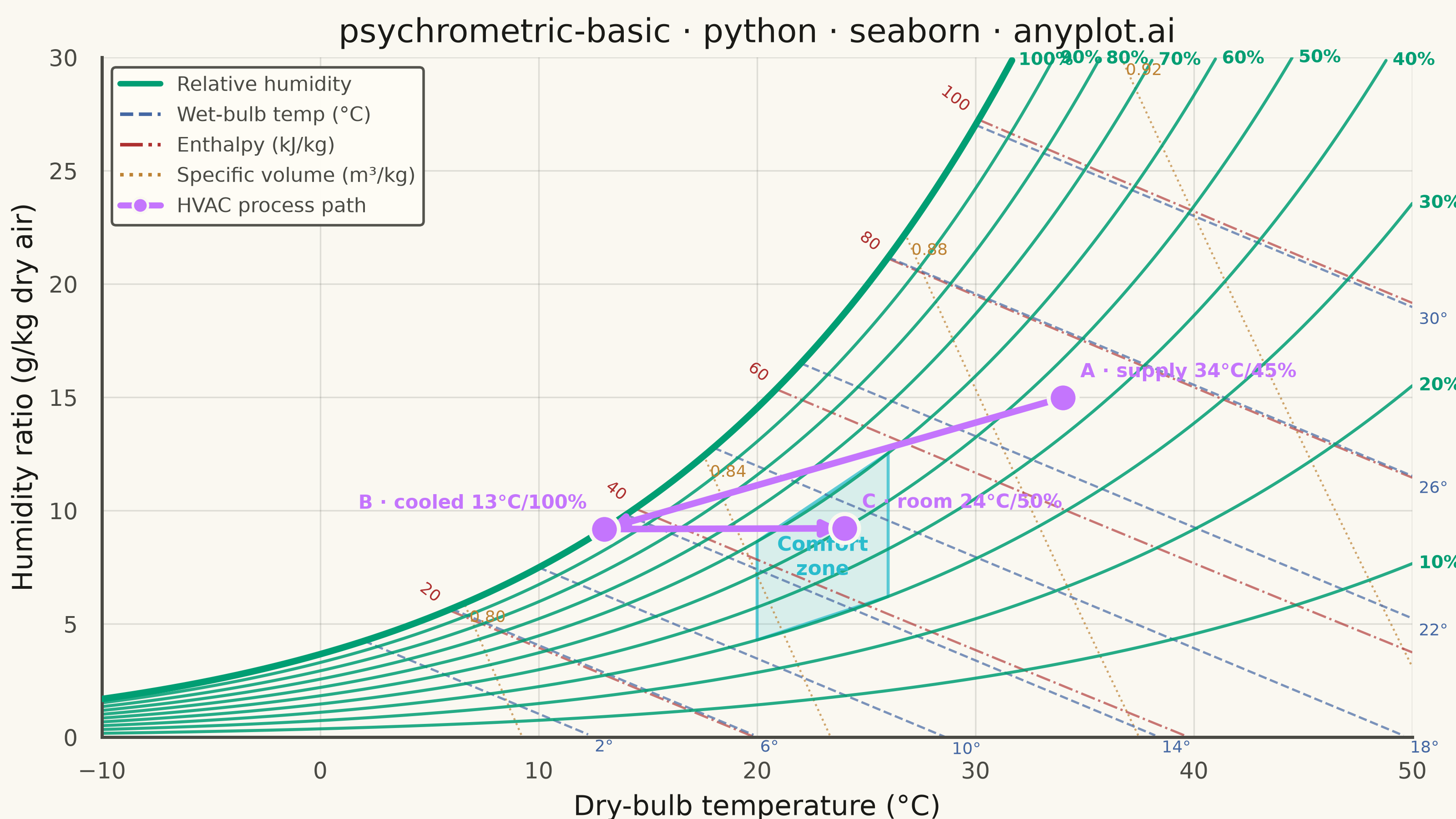
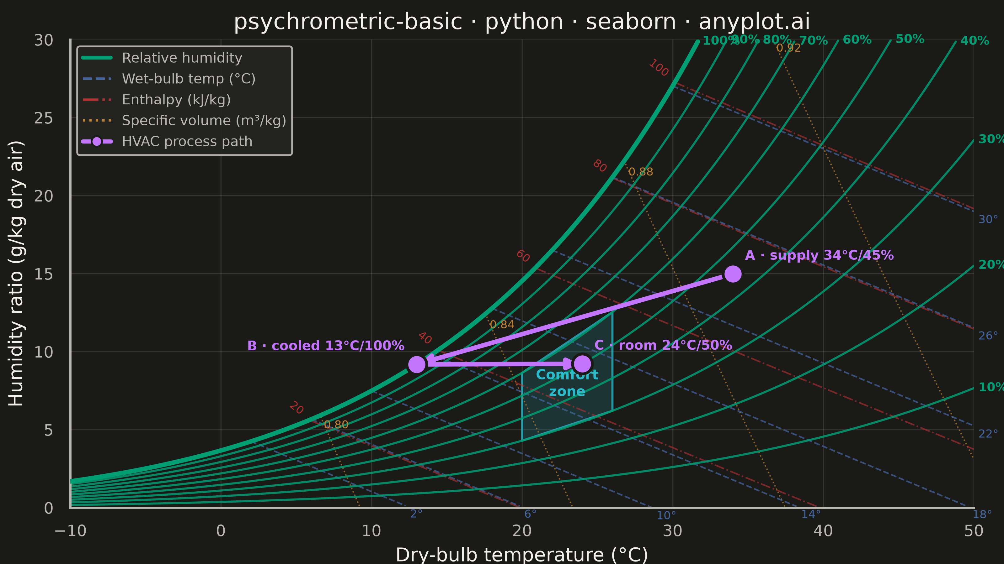
A psychrometric chart plots dry-bulb temperature against humidity ratio, overlaid with curves for relative humidity, wet-bulb temperature, enthalpy, and specific volume. It is the fundamental tool for HVAC system design and air conditioning process analysis. The chart reveals the thermodynamic properties of moist air at a glance, enabling engineers to trace heating, cooling, humidification, and dehumidification processes as paths on the diagram.
""" anyplot.ai
psychrometric-basic: Psychrometric Chart for HVAC
Library: seaborn 0.13.2 | Python 3.13.14
Quality: 90/100 | Updated: 2026-06-16
"""

import os

import matplotlib.pyplot as plt
import numpy as np
import pandas as pd
import seaborn as sns
from matplotlib.lines import Line2D


# Theme-adaptive chrome (see prompts/default-style-guide.md "Theme-adaptive Chrome")
THEME = os.getenv("ANYPLOT_THEME", "light")
PAGE_BG = "#FAF8F1" if THEME == "light" else "#1A1A17"
ELEVATED_BG = "#FFFDF6" if THEME == "light" else "#242420"
INK = "#1A1A17" if THEME == "light" else "#F0EFE8"
INK_SOFT = "#4A4A44" if THEME == "light" else "#B8B7B0"

# Imprint palette — first family is brand green, then canonical order; line styles
# reinforce colour for colourblind safety.
RH_COLOR = "#009E73"  # brand green — relative-humidity curves (most prominent family)
WB_COLOR = "#4467A3"  # blue — wet-bulb isotherms
ENTH_COLOR = "#AE3030"  # matte red — constant enthalpy (energy)
SV_COLOR = "#BD8233"  # ochre — constant specific volume
COMFORT_COLOR = "#2ABCCD"  # cyan — comfort-zone region
PROCESS_COLOR = "#C475FD"  # lavender — HVAC process path

# Data — moist-air properties at standard sea-level pressure (101.325 kPa)
np.random.seed(42)
P_ATM = 101325  # Pa
T_GRID = np.linspace(-10, 50, 600)

# Saturation vapour pressure (Pa) and saturation humidity ratio (g/kg) over water
# (ASHRAE) — a single continuous relation across the whole range keeps the curves
# smooth (no kink at 0 °C).
P_SAT = np.exp(23.196 - 3816.44 / (T_GRID + 227.02))
W_SAT = 0.62198 * P_SAT / (P_ATM - P_SAT) * 1000

# Constant relative-humidity curves (10% – 100%)
rh_rows = []
for rh in np.arange(10, 101, 10):
    p_v = (rh / 100) * P_SAT
    w = 0.62198 * p_v / (P_ATM - p_v) * 1000
    keep = (w >= 0) & (w <= 30)
    for t, wv in zip(T_GRID[keep], w[keep], strict=True):
        rh_rows.append({"t": t, "w": wv, "rh": f"{rh}%"})
rh_df = pd.DataFrame(rh_rows)

# Constant wet-bulb isotherms (line slope ≈ -0.402 g/kg per °C)
wb_rows = []
for t_wb in np.arange(2, 31, 4):
    w0 = float(np.interp(t_wb, T_GRID, W_SAT))
    t_line = np.linspace(t_wb, 50, 160)
    w_line = w0 - 0.402 * (t_line - t_wb)
    cap = np.minimum(np.interp(t_line, T_GRID, W_SAT), 30)
    keep = (w_line >= 0) & (w_line <= cap)
    for t, wv in zip(t_line[keep], w_line[keep], strict=True):
        wb_rows.append({"t": t, "w": wv, "twb": f"{t_wb}"})
wb_df = pd.DataFrame(wb_rows)

# Constant enthalpy lines (kJ/kg dry air)
enth_rows = []
for h in np.arange(20, 101, 20):
    w_line = (h - 1.006 * T_GRID) / (2.501 + 0.00186 * T_GRID)
    keep = (w_line >= 0) & (w_line <= np.minimum(W_SAT, 30))
    for t, wv in zip(T_GRID[keep], w_line[keep], strict=True):
        enth_rows.append({"t": t, "w": wv, "h": f"{h}"})
enth_df = pd.DataFrame(enth_rows)

# Constant specific-volume lines (m³/kg dry air)
sv_rows = []
for v in np.arange(0.80, 0.93, 0.04):
    w_line = ((v * P_ATM / 1000) / (0.287042 * (T_GRID + 273.15)) - 1) / 1.6078 * 1000
    keep = (w_line >= 0) & (w_line <= np.minimum(W_SAT, 30))
    for t, wv in zip(T_GRID[keep], w_line[keep], strict=True):
        sv_rows.append({"t": t, "w": wv, "v": f"{v:.2f}"})
sv_df = pd.DataFrame(sv_rows)

# Comfort zone (≈20–26 °C, 30–60% RH) and a cooling + dehumidification process path
comfort_t = np.array([20, 26, 26, 20])
comfort_w = np.array(
    [
        0.62198 * (0.30 * np.interp(20, T_GRID, P_SAT)) / (P_ATM - 0.30 * np.interp(20, T_GRID, P_SAT)) * 1000,
        0.62198 * (0.30 * np.interp(26, T_GRID, P_SAT)) / (P_ATM - 0.30 * np.interp(26, T_GRID, P_SAT)) * 1000,
        0.62198 * (0.60 * np.interp(26, T_GRID, P_SAT)) / (P_ATM - 0.60 * np.interp(26, T_GRID, P_SAT)) * 1000,
        0.62198 * (0.60 * np.interp(20, T_GRID, P_SAT)) / (P_ATM - 0.60 * np.interp(20, T_GRID, P_SAT)) * 1000,
    ]
)

state_points = pd.DataFrame(
    {
        "t": [34.0, 13.0, 24.0],
        "w": [
            0.62198 * (0.45 * np.interp(34, T_GRID, P_SAT)) / (P_ATM - 0.45 * np.interp(34, T_GRID, P_SAT)) * 1000,
            float(np.interp(13, T_GRID, W_SAT)),
            0.62198 * (0.50 * np.interp(24, T_GRID, P_SAT)) / (P_ATM - 0.50 * np.interp(24, T_GRID, P_SAT)) * 1000,
        ],
        "label": ["A · supply 34°C/45%", "B · cooled 13°C/100%", "C · room 24°C/50%"],
    }
)

# Plot — 16:9 canvas (8 × 4.5 in @ dpi=400 → 3200 × 1800 px)
sns.set_theme(
    style="whitegrid",
    rc={
        "figure.facecolor": PAGE_BG,
        "axes.facecolor": PAGE_BG,
        "axes.edgecolor": INK_SOFT,
        "axes.labelcolor": INK,
        "text.color": INK,
        "xtick.color": INK_SOFT,
        "ytick.color": INK_SOFT,
        "grid.color": INK,
        "grid.alpha": 0.12,
        "grid.linewidth": 0.6,
        "font.family": "sans-serif",
    },
)
fig, ax = plt.subplots(figsize=(8, 4.5), dpi=400)

# Comfort zone sits behind the property lines
ax.fill(comfort_t, comfort_w, color=COMFORT_COLOR, alpha=0.16, zorder=1)
ax.plot(
    np.append(comfort_t, comfort_t[0]),
    np.append(comfort_w, comfort_w[0]),
    color=COMFORT_COLOR,
    linewidth=1.2,
    alpha=0.7,
    zorder=1,
)

# Property-line families, each drawn as one seaborn lineplot (units → one line per level)
sns.lineplot(
    data=sv_df,
    x="t",
    y="w",
    units="v",
    estimator=None,
    color=SV_COLOR,
    linewidth=0.8,
    linestyle=":",
    alpha=0.7,
    ax=ax,
    legend=False,
)
sns.lineplot(
    data=enth_df,
    x="t",
    y="w",
    units="h",
    estimator=None,
    color=ENTH_COLOR,
    linewidth=0.9,
    linestyle="-.",
    alpha=0.65,
    ax=ax,
    legend=False,
)
sns.lineplot(
    data=wb_df,
    x="t",
    y="w",
    units="twb",
    estimator=None,
    color=WB_COLOR,
    linewidth=0.9,
    linestyle="--",
    alpha=0.7,
    ax=ax,
    legend=False,
)
sns.lineplot(
    data=rh_df, x="t", y="w", units="rh", estimator=None, color=RH_COLOR, linewidth=1.2, alpha=0.85, ax=ax, legend=False
)

# Saturation curve (100% RH) — prominent upper boundary
sat = rh_df[rh_df["rh"] == "100%"]
ax.plot(sat["t"], sat["w"], color=RH_COLOR, linewidth=2.6, zorder=4)

# HVAC process path: cooling + dehumidification (A→B), then sensible reheat (B→C)
for i in range(2):
    ax.annotate(
        "",
        xy=(state_points["t"][i + 1], state_points["w"][i + 1]),
        xytext=(state_points["t"][i], state_points["w"][i]),
        arrowprops={"arrowstyle": "-|>", "color": PROCESS_COLOR, "lw": 2.6},
        zorder=5,
    )
sns.scatterplot(
    data=state_points,
    x="t",
    y="w",
    color=PROCESS_COLOR,
    s=130,
    edgecolor=PAGE_BG,
    linewidth=1.6,
    zorder=6,
    legend=False,
    ax=ax,
)

# Direct labels (spec: label property lines on the chart) — spread to edges to avoid crowding
for rh in rh_df["rh"].unique():
    seg = rh_df[rh_df["rh"] == rh]
    ax.text(
        float(seg["t"].iloc[-1]) + 0.3,
        float(seg["w"].iloc[-1]),
        rh,
        fontsize=7,
        color=RH_COLOR,
        ha="left",
        va="center",
        fontweight="bold",
    )
for twb in wb_df["twb"].unique():
    seg = wb_df[wb_df["twb"] == twb]
    ax.text(
        float(seg["t"].iloc[-1]) + 0.3,
        float(seg["w"].iloc[-1]) - 0.2,
        f"{twb}°",
        fontsize=6.5,
        color=WB_COLOR,
        ha="left",
        va="top",
    )
for h in enth_df["h"].unique():
    seg = enth_df[enth_df["h"] == h]
    ax.text(
        float(seg["t"].iloc[0]) - 0.3,
        float(seg["w"].iloc[0]) + 0.2,
        h,
        fontsize=6.5,
        color=ENTH_COLOR,
        ha="right",
        va="bottom",
        rotation=-38,
    )
for v in sv_df["v"].unique():
    seg = sv_df[sv_df["v"] == v]
    ax.text(
        float(seg["t"].iloc[0]) + 0.2,
        float(seg["w"].iloc[0]) - 0.2,
        v,
        fontsize=6.5,
        color=SV_COLOR,
        ha="left",
        va="top",
    )

ax.text(
    23,
    float(comfort_w.mean()),
    "Comfort\nzone",
    fontsize=8,
    color=COMFORT_COLOR,
    ha="center",
    va="center",
    fontweight="bold",
)
for _, row in state_points.iterrows():
    dx = -0.8 if row["label"].startswith("B") else 0.8
    ha = "right" if row["label"].startswith("B") else "left"
    ax.text(
        row["t"] + dx,
        row["w"] + 0.7,
        row["label"],
        fontsize=7.5,
        color=PROCESS_COLOR,
        ha=ha,
        va="bottom",
        fontweight="bold",
    )

# Legend — sits in the empty upper-left zone (cold + humid is physically unreachable)
legend_handles = [
    Line2D([0], [0], color=RH_COLOR, lw=2.2, label="Relative humidity"),
    Line2D([0], [0], color=WB_COLOR, lw=1.4, ls="--", label="Wet-bulb temp (°C)"),
    Line2D([0], [0], color=ENTH_COLOR, lw=1.4, ls="-.", label="Enthalpy (kJ/kg)"),
    Line2D([0], [0], color=SV_COLOR, lw=1.4, ls=":", label="Specific volume (m³/kg)"),
    Line2D(
        [0],
        [0],
        color=PROCESS_COLOR,
        lw=2.4,
        marker="o",
        markersize=6,
        markeredgecolor=PAGE_BG,
        label="HVAC process path",
    ),
]
legend = ax.legend(
    handles=legend_handles, loc="upper left", fontsize=8, framealpha=0.95, facecolor=ELEVATED_BG, edgecolor=INK_SOFT
)
legend.get_title().set_color(INK)
for text in legend.get_texts():
    text.set_color(INK_SOFT)

# Style
ax.set_xlim(-10, 50)
ax.set_ylim(0, 30)
ax.set_xlabel("Dry-bulb temperature (°C)", fontsize=11, color=INK)
ax.set_ylabel("Humidity ratio (g/kg dry air)", fontsize=11, color=INK)
ax.set_title("psychrometric-basic · python · seaborn · anyplot.ai", fontsize=13, fontweight="medium", color=INK)
ax.tick_params(axis="both", labelsize=9, colors=INK_SOFT)
sns.despine(ax=ax)

# Save
fig.subplots_adjust(left=0.07, right=0.97, top=0.93, bottom=0.1)
plt.savefig(f"plot-{THEME}.png", dpi=400, facecolor=PAGE_BG)
Runnable source as JSON, for any HTTP client: https://api.anyplot.ai/specs/psychrometric-basic/seaborn/code. Any spec id and library id listed in llms-full.txt fit the same URL shape; every URL below is complete and callable.
{
  "spec_id": "psychrometric-basic",
  "language": "python",
  "library": "seaborn",
  "page": "https://anyplot.ai/psychrometric-basic/python/seaborn",
  "hub": "https://anyplot.ai/psychrometric-basic",
  "code_json": "https://api.anyplot.ai/specs/psychrometric-basic/seaborn/code",
  "spec_json": "https://api.anyplot.ai/specs/psychrometric-basic",
  "render_light_png": "https://storage.googleapis.com/anyplot-images/plots/psychrometric-basic/python/seaborn/plot-light.png",
  "render_dark_png": "https://storage.googleapis.com/anyplot-images/plots/psychrometric-basic/python/seaborn/plot-dark.png",
  "quality_score": 90.0,
  "license": "MIT",
  "guide": "https://anyplot.ai/llms.txt"
}
Part of Psychrometric Chart for HVAC on anyplot.ai.