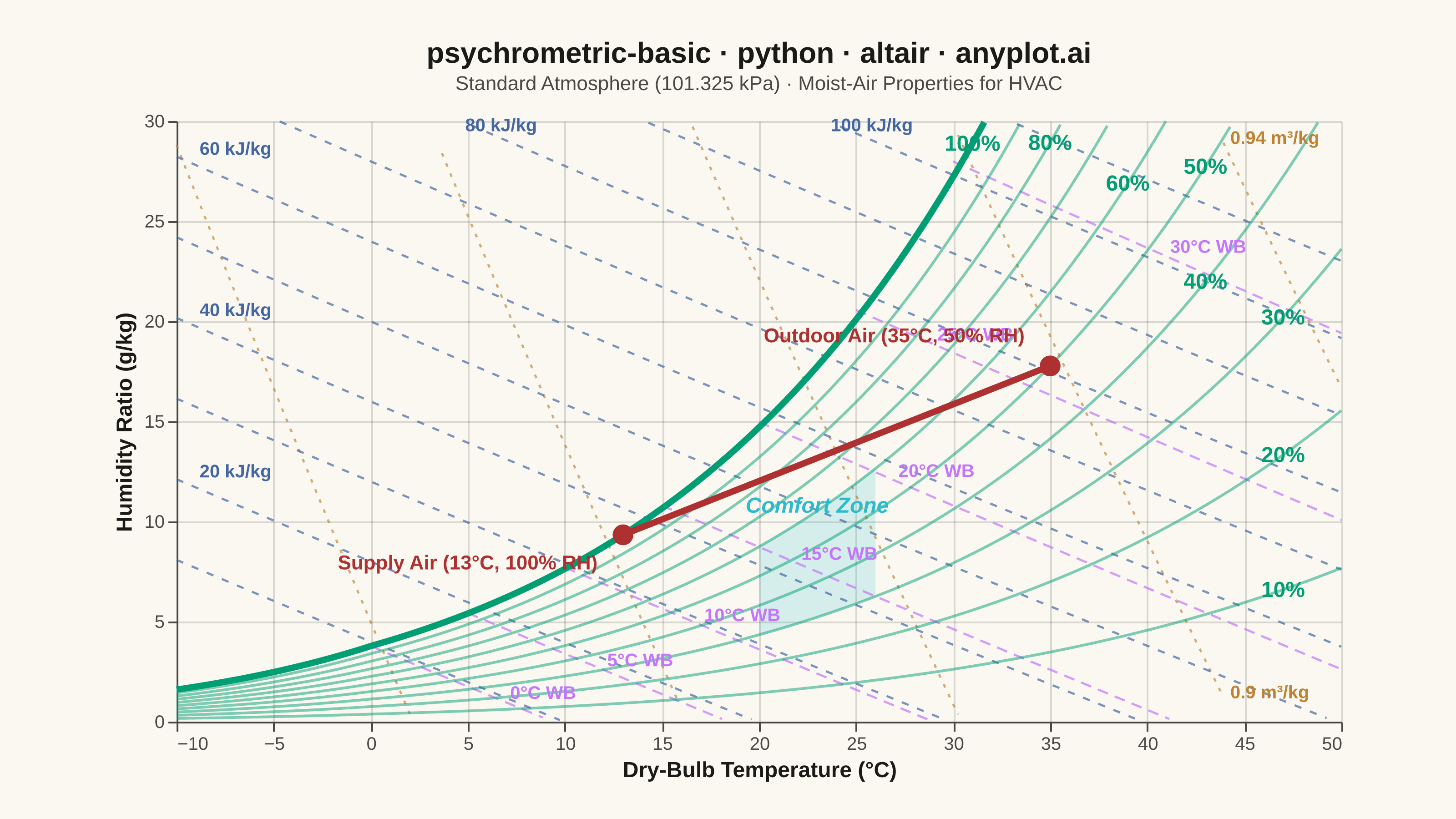
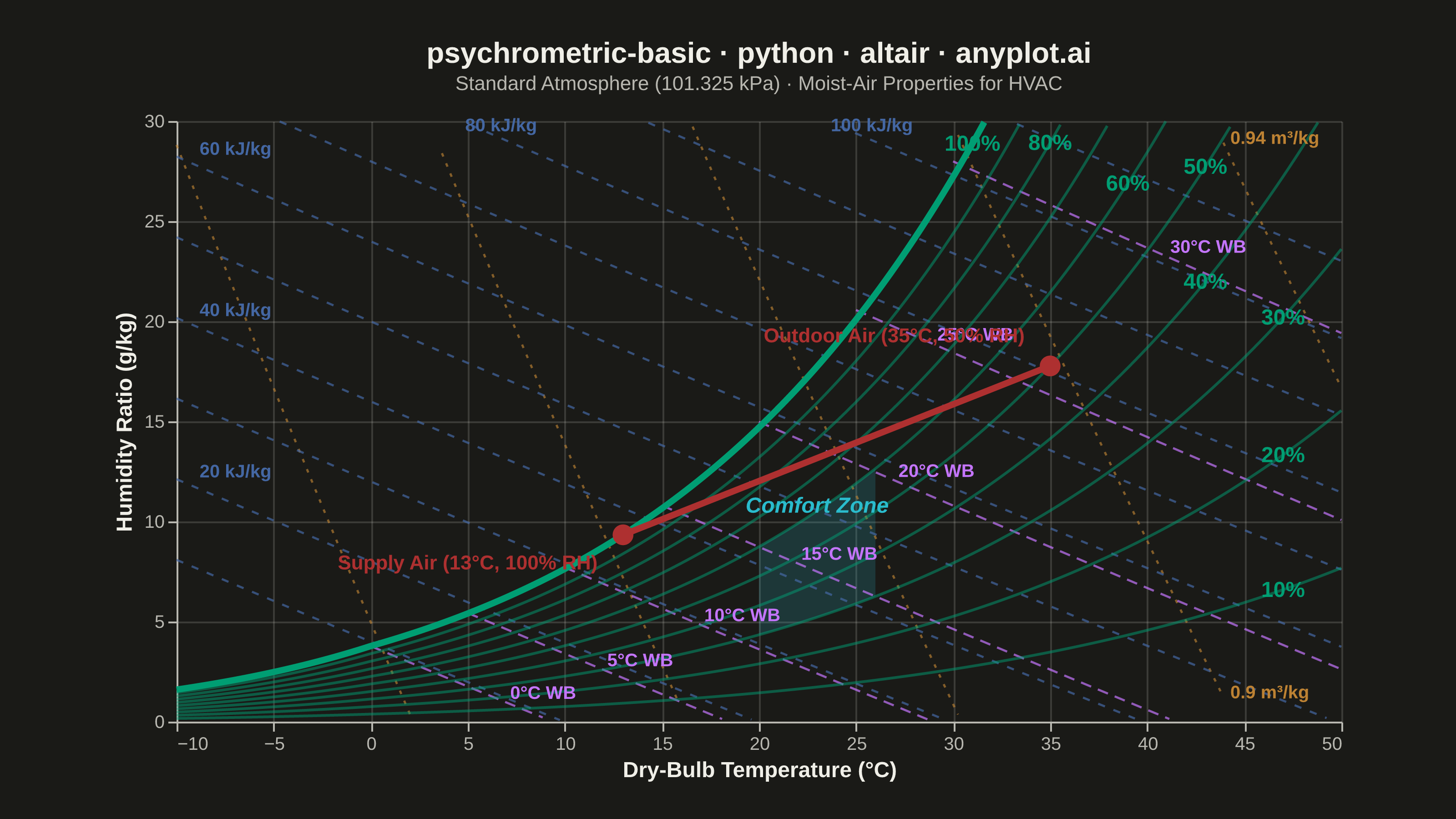
A psychrometric chart plots dry-bulb temperature against humidity ratio, overlaid with curves for relative humidity, wet-bulb temperature, enthalpy, and specific volume. It is the fundamental tool for HVAC system design and air conditioning process analysis. The chart reveals the thermodynamic properties of moist air at a glance, enabling engineers to trace heating, cooling, humidification, and dehumidification processes as paths on the diagram.
""" anyplot.ai
psychrometric-basic: Psychrometric Chart for HVAC
Library: altair 6.2.1 | Python 3.13.13
Quality: 86/100 | Updated: 2026-06-16
"""

import os
import sys


# Strip the script directory from sys.path so `import altair` resolves to the
# installed package, not this file (which is named altair.py).
_script_dir = os.path.dirname(os.path.abspath(__file__))
sys.path[:] = [p for p in sys.path if os.path.abspath(p or ".") != _script_dir]

import altair as alt
import numpy as np
import pandas as pd
from PIL import Image


# Theme tokens (see prompts/default-style-guide.md "Theme-adaptive Chrome")
THEME = os.getenv("ANYPLOT_THEME", "light")
PAGE_BG = "#FAF8F1" if THEME == "light" else "#1A1A17"
INK = "#1A1A17" if THEME == "light" else "#F0EFE8"
INK_SOFT = "#4A4A44" if THEME == "light" else "#B8B7B0"

# Imprint palette — each moist-air property family gets one canonical hue.
CLR_RH = "#009E73"  # brand green — relative humidity + saturation (first series)
CLR_WB = "#C475FD"  # lavender — wet-bulb temperature lines
CLR_ENTHALPY = "#4467A3"  # blue — constant enthalpy lines
CLR_VOL = "#BD8233"  # ochre — constant specific-volume lines
CLR_PROCESS = "#AE3030"  # matte red (semantic emphasis) — HVAC process path
CLR_COMFORT = "#2ABCCD"  # cyan — thermal comfort zone

# Constants
P_ATM = 101325  # Pa, standard sea-level atmospheric pressure

# Saturation pressure over a fine grid (ASHRAE 2017 formula), computed once.
_t_grid = np.linspace(-10, 50, 500)
_t_grid_k = _t_grid + 273.15
_p_sat_grid = np.where(
    _t_grid >= 0,
    np.exp(
        -5.8002206e3 / _t_grid_k
        + 1.3914993
        - 4.8640239e-2 * _t_grid_k
        + 4.1764768e-5 * _t_grid_k**2
        - 1.4452093e-8 * _t_grid_k**3
        + 6.5459673 * np.log(_t_grid_k)
    ),
    np.exp(
        -5.6745359e3 / _t_grid_k
        + 6.3925247
        - 9.677843e-3 * _t_grid_k
        + 6.2215701e-7 * _t_grid_k**2
        + 2.0747825e-9 * _t_grid_k**3
        - 9.484024e-13 * _t_grid_k**4
        + 4.1635019 * np.log(_t_grid_k)
    ),
)

# Data — psychrometric property curves over the -10..50 °C dry-bulb range.
t_range = np.linspace(-10, 50, 200)
p_sat = np.interp(t_range, _t_grid, _p_sat_grid)

# Relative-humidity curves (10% to 100%)
rh_curves = []
for rh_pct in range(10, 110, 10):
    p_w = (rh_pct / 100) * p_sat
    w_vals = 0.621945 * p_w / (P_ATM - p_w) * 1000  # g/kg
    for t, w in zip(t_range, w_vals, strict=True):
        if 0 < w <= 30:
            rh_curves.append({"t_db": float(t), "w": float(w), "rh": f"{rh_pct}%"})

rh_df = pd.DataFrame(rh_curves)

# Wet-bulb temperature lines (constant t_wb)
wb_lines = []
for t_wb_val in range(0, 36, 5):
    p_sat_wb = float(np.interp(t_wb_val, _t_grid, _p_sat_grid))
    w_s_wb = 0.621945 * p_sat_wb / (P_ATM - p_sat_wb)
    for t_db in np.linspace(t_wb_val, 50, 80):
        w = (2501 * w_s_wb - 1.006 * (t_db - t_wb_val)) / (2501 + 1.86 * t_db - 4.186 * t_wb_val)
        w_gkg = w * 1000
        if 0 <= w_gkg <= 30:
            wb_lines.append({"t_db": float(t_db), "w": float(w_gkg), "wb": f"{t_wb_val}°C"})

wb_df = pd.DataFrame(wb_lines)

# Constant-enthalpy lines (h = 1.006*t + w*(2501 + 1.86*t), solved for w)
enthalpy_lines = []
for h_val in range(10, 120, 10):
    for t_db in np.linspace(-10, 50, 80):
        w_gkg = (h_val - 1.006 * t_db) / (2.501 + 0.00186 * t_db)
        if 0 <= w_gkg <= 30:
            enthalpy_lines.append({"t_db": float(t_db), "w": float(w_gkg), "h": f"{h_val} kJ/kg"})

enthalpy_df = pd.DataFrame(enthalpy_lines)

# Constant specific-volume lines (v = 0.287042*T_k*(1+1.6078*w)/P, solved for w)
vol_lines = []
for v_val in [0.78, 0.82, 0.86, 0.90, 0.94]:
    for t_db in np.linspace(-10, 50, 80):
        w = (v_val * P_ATM / 1000 / (0.287042 * (t_db + 273.15)) - 1) / 1.6078
        w_gkg = w * 1000
        if 0 <= w_gkg <= 30:
            vol_lines.append({"t_db": float(t_db), "w": float(w_gkg), "v": f"{v_val} m³/kg"})

vol_df = pd.DataFrame(vol_lines)

# Comfort zone (20-26 °C, 30-60% RH)
comfort_temps = np.linspace(20, 26, 30)
comfort_psat = np.interp(comfort_temps, _t_grid, _p_sat_grid)
comfort_w_lo = 0.621945 * 0.30 * comfort_psat / (P_ATM - 0.30 * comfort_psat) * 1000
comfort_w_hi = 0.621945 * 0.60 * comfort_psat / (P_ATM - 0.60 * comfort_psat) * 1000
comfort_df = pd.DataFrame({"t_db": comfort_temps, "w": comfort_w_lo, "w2": comfort_w_hi})

# HVAC process path: cooling + dehumidification (35 °C/50% RH -> 13 °C/saturated)
t1, t2 = 35.0, 13.0
p_sat_t1, p_sat_t2 = float(np.interp(t1, _t_grid, _p_sat_grid)), float(np.interp(t2, _t_grid, _p_sat_grid))
w1 = 0.621945 * 0.50 * p_sat_t1 / (P_ATM - 0.50 * p_sat_t1) * 1000
w2 = 0.621945 * 1.00 * p_sat_t2 / (P_ATM - 1.00 * p_sat_t2) * 1000

process_points = pd.DataFrame(
    {
        "t_db": [t1, t2],
        "w": [float(w1), float(w2)],
        "label": ["Outdoor Air (35°C, 50% RH)", "Supply Air (13°C, 100% RH)"],
        "rh_pct": ["50%", "100%"],
        "order": [0, 1],
    }
)

# RH labels — staggered along the curves to avoid convergence overlap near saturation
rh_labels = []
for rh_pct in range(10, 110, 10):
    if rh_pct == 100:
        t_label = 31
    elif rh_pct >= 80:
        t_label = 35
    elif rh_pct >= 60:
        t_label = 39
    elif rh_pct >= 40:
        t_label = 43
    else:
        t_label = 47
    p_sat_label = float(np.interp(t_label, _t_grid, _p_sat_grid))
    w_label = 0.621945 * (rh_pct / 100) * p_sat_label / (P_ATM - (rh_pct / 100) * p_sat_label) * 1000
    if w_label <= 30:
        rh_labels.append({"t_db": float(t_label), "w": float(w_label), "label": f"{rh_pct}%"})

rh_label_df = pd.DataFrame(rh_labels)

# Wet-bulb labels — placed in the interior along each line, away from the saturation crowd.
# Per-line anchor offsets: 25 °C steps left to clear the red process marker (~35 °C, 17.8 g/kg);
# 30 °C steps right to descend out of the crowded saturation apex.
wb_label_offset = {25: 4, 30: 11}
wb_labels_data = []
for t_wb_val in range(0, 36, 5):
    p_sat_wb = float(np.interp(t_wb_val, _t_grid, _p_sat_grid))
    w_s_wb = 0.621945 * p_sat_wb / (P_ATM - p_sat_wb)
    t_at = t_wb_val + wb_label_offset.get(t_wb_val, 7)
    w_at = (2501 * w_s_wb - 1.006 * (t_at - t_wb_val)) / (2501 + 1.86 * t_at - 4.186 * t_wb_val) * 1000
    if 0 < w_at <= 28:
        wb_labels_data.append({"t_db": float(t_at), "w": float(w_at), "label": f"{t_wb_val}°C WB"})

wb_label_df = pd.DataFrame(wb_labels_data)

# Enthalpy labels — anchored on the left/top edges where wet-bulb labels are absent
enthalpy_labels = []
for h_val in range(20, 120, 20):
    w_at_left = (h_val - 1.006 * (-10)) / (2.501 + 0.00186 * (-10))
    if 0 <= w_at_left <= 30:
        enthalpy_labels.append({"t_db": -9.0, "w": float(w_at_left), "label": f"{h_val} kJ/kg"})
    else:
        t_at_top = (h_val - 2.501 * 30) / (1.006 + 0.00186 * 30)
        if -10 <= t_at_top <= 50:
            enthalpy_labels.append({"t_db": float(t_at_top), "w": 29.4, "label": f"{h_val} kJ/kg"})

enthalpy_label_df = pd.DataFrame(enthalpy_labels)

# Volume labels — along the lower-right where the volume lines exit the frame
vol_labels = []
for v_val in [0.78, 0.82, 0.86, 0.90, 0.94]:
    w_at = (v_val * P_ATM / 1000 / (0.287042 * (44 + 273.15)) - 1) / 1.6078 * 1000
    if 0 <= w_at <= 30:
        vol_labels.append({"t_db": 44.0, "w": float(w_at), "label": f"{v_val} m³/kg"})

vol_label_df = pd.DataFrame(vol_labels)

# Plot
x_scale = alt.Scale(domain=[-10, 50])
y_scale = alt.Scale(domain=[0, 30])

# Comfort zone shaded band
comfort = (
    alt.Chart(comfort_df)
    .mark_area(opacity=0.18, color=CLR_COMFORT)
    .encode(x=alt.X("t_db:Q", scale=x_scale), y=alt.Y("w:Q", scale=y_scale), y2="w2:Q")
)

comfort_label = (
    alt.Chart(pd.DataFrame({"t_db": [23.0], "w": [10.8], "label": ["Comfort Zone"]}))
    .mark_text(fontSize=12, color=CLR_COMFORT, fontWeight="bold", fontStyle="italic")
    .encode(x=alt.X("t_db:Q", scale=x_scale), y=alt.Y("w:Q", scale=y_scale), text="label:N")
)

# Specific-volume lines (ochre)
vol_chart = (
    alt.Chart(vol_df)
    .mark_line(strokeWidth=1.2, strokeDash=[2, 4], opacity=0.65, color=CLR_VOL)
    .encode(x=alt.X("t_db:Q", scale=x_scale), y=alt.Y("w:Q", scale=y_scale), detail="v:N")
)

vol_text = (
    alt.Chart(vol_label_df)
    .mark_text(fontSize=10, color=CLR_VOL, align="left", dx=3, dy=-4, fontWeight="bold")
    .encode(x=alt.X("t_db:Q", scale=x_scale), y=alt.Y("w:Q", scale=y_scale), text="label:N")
)

# Constant-enthalpy lines (blue)
enthalpy_chart = (
    alt.Chart(enthalpy_df)
    .mark_line(strokeWidth=1.2, strokeDash=[4, 5], opacity=0.7, color=CLR_ENTHALPY)
    .encode(x=alt.X("t_db:Q", scale=x_scale), y=alt.Y("w:Q", scale=y_scale), detail="h:N")
)

enthalpy_text = (
    alt.Chart(enthalpy_label_df)
    .mark_text(fontSize=10, color=CLR_ENTHALPY, align="left", dx=2, dy=-4, fontWeight="bold")
    .encode(x=alt.X("t_db:Q", scale=x_scale), y=alt.Y("w:Q", scale=y_scale), text="label:N")
)

# Wet-bulb lines (lavender)
wb_chart = (
    alt.Chart(wb_df)
    .mark_line(strokeWidth=1.2, strokeDash=[6, 4], opacity=0.7, color=CLR_WB)
    .encode(
        x=alt.X("t_db:Q", scale=x_scale),
        y=alt.Y("w:Q", scale=y_scale),
        detail="wb:N",
        tooltip=[
            alt.Tooltip("t_db:Q", title="Dry-Bulb (°C)", format=".1f"),
            alt.Tooltip("w:Q", title="Humidity (g/kg)", format=".1f"),
            alt.Tooltip("wb:N", title="Wet-Bulb Temp"),
        ],
    )
)

wb_text = (
    alt.Chart(wb_label_df)
    .mark_text(fontSize=10, color=CLR_WB, align="left", dx=2, dy=-5, fontWeight="bold")
    .encode(x=alt.X("t_db:Q", scale=x_scale), y=alt.Y("w:Q", scale=y_scale), text="label:N")
)

# Relative-humidity curves (10%-90%, brand green, lighter than saturation)
other_rh_df = rh_df[rh_df["rh"] != "100%"]
rh_chart = (
    alt.Chart(other_rh_df)
    .mark_line(strokeWidth=1.5, opacity=0.5, color=CLR_RH)
    .encode(
        x=alt.X("t_db:Q", scale=x_scale),
        y=alt.Y("w:Q", scale=y_scale),
        detail="rh:N",
        tooltip=[
            alt.Tooltip("t_db:Q", title="Dry-Bulb (°C)", format=".1f"),
            alt.Tooltip("w:Q", title="Humidity (g/kg)", format=".1f"),
            alt.Tooltip("rh:N", title="Relative Humidity"),
        ],
    )
)

# Saturation curve (100% RH) — the prominent upper boundary
sat_df = rh_df[rh_df["rh"] == "100%"]
saturation = (
    alt.Chart(sat_df)
    .mark_line(strokeWidth=3.5, color=CLR_RH)
    .encode(
        x=alt.X("t_db:Q", scale=x_scale, title="Dry-Bulb Temperature (°C)"),
        y=alt.Y("w:Q", scale=y_scale, title="Humidity Ratio (g/kg)"),
    )
)

rh_text = (
    alt.Chart(rh_label_df)
    .mark_text(fontSize=12, color=CLR_RH, fontWeight="bold")
    .encode(x=alt.X("t_db:Q", scale=x_scale), y=alt.Y("w:Q", scale=y_scale), text="label:N")
)

# HVAC process path (matte red) — focal point with state-point markers
process_line = (
    alt.Chart(process_points)
    .mark_line(strokeWidth=3.5, color=CLR_PROCESS, point=alt.OverlayMarkDef(size=130, filled=True, color=CLR_PROCESS))
    .encode(
        x=alt.X("t_db:Q", scale=x_scale),
        y=alt.Y("w:Q", scale=y_scale),
        order="order:Q",
        tooltip=[
            alt.Tooltip("label:N", title="State Point"),
            alt.Tooltip("t_db:Q", title="Dry-Bulb (°C)", format=".1f"),
            alt.Tooltip("w:Q", title="Humidity (g/kg)", format=".1f"),
            alt.Tooltip("rh_pct:N", title="RH"),
        ],
    )
)

outdoor_label = (
    alt.Chart(process_points[process_points["order"] == 0])
    .mark_text(fontSize=11, fontWeight="bold", color=CLR_PROCESS, align="right", dx=-14, dy=-16)
    .encode(x=alt.X("t_db:Q", scale=x_scale), y=alt.Y("w:Q", scale=y_scale), text="label:N")
)

supply_label = (
    alt.Chart(process_points[process_points["order"] == 1])
    .mark_text(fontSize=11, fontWeight="bold", color=CLR_PROCESS, align="right", dx=-14, dy=16)
    .encode(x=alt.X("t_db:Q", scale=x_scale), y=alt.Y("w:Q", scale=y_scale), text="label:N")
)

# Layer all elements (faint property grids first, prominent features last)
chart = (
    alt.layer(
        comfort,
        vol_chart,
        enthalpy_chart,
        wb_chart,
        rh_chart,
        saturation,
        vol_text,
        enthalpy_text,
        wb_text,
        rh_text,
        comfort_label,
        process_line,
        outdoor_label,
        supply_label,
    )
    .properties(
        width=640,
        height=330,
        background=PAGE_BG,
        title=alt.Title(
            text="psychrometric-basic · python · altair · anyplot.ai",
            fontSize=16,
            anchor="middle",
            color=INK,
            subtitle="Standard Atmosphere (101.325 kPa) · Moist-Air Properties for HVAC",
            subtitleFontSize=11,
            subtitleColor=INK_SOFT,
            offset=10,
        ),
    )
    .configure_view(strokeWidth=0, fill=PAGE_BG)
    .configure_axis(
        labelFontSize=10,
        titleFontSize=12,
        titleColor=INK,
        labelColor=INK_SOFT,
        grid=True,
        gridOpacity=0.15,
        gridColor=INK,
        domainColor=INK_SOFT,
        tickColor=INK_SOFT,
    )
)

# Save — interactive HTML untouched; PNG padded to the exact canonical target.
chart.save(f"plot-{THEME}.html")
chart.save(f"plot-{THEME}.png", scale_factor=4.0)

TW, TH = 3200, 1800
_img = Image.open(f"plot-{THEME}.png").convert("RGB")
_w, _h = _img.size
if _w > TW or _h > TH:
    raise SystemExit(
        f"altair vl-convert produced {_w}×{_h}, exceeds target {TW}×{TH}. "
        f"Shrink chart .properties(width=, height=) values and re-render."
    )
if _w < TW or _h < TH:
    _canvas = Image.new("RGB", (TW, TH), PAGE_BG)
    _canvas.paste(_img, ((TW - _w) // 2, (TH - _h) // 2))
    _canvas.save(f"plot-{THEME}.png")
Runnable source as JSON, for any HTTP client: https://api.anyplot.ai/specs/psychrometric-basic/altair/code. Any spec id and library id listed in llms-full.txt fit the same URL shape; every URL below is complete and callable.
{
  "spec_id": "psychrometric-basic",
  "language": "python",
  "library": "altair",
  "page": "https://anyplot.ai/psychrometric-basic/python/altair",
  "hub": "https://anyplot.ai/psychrometric-basic",
  "code_json": "https://api.anyplot.ai/specs/psychrometric-basic/altair/code",
  "spec_json": "https://api.anyplot.ai/specs/psychrometric-basic",
  "render_light_png": "https://storage.googleapis.com/anyplot-images/plots/psychrometric-basic/python/altair/plot-light.png",
  "render_dark_png": "https://storage.googleapis.com/anyplot-images/plots/psychrometric-basic/python/altair/plot-dark.png",
  "interactive_light_html": "https://storage.googleapis.com/anyplot-images/plots/psychrometric-basic/python/altair/plot-light.html",
  "interactive_dark_html": "https://storage.googleapis.com/anyplot-images/plots/psychrometric-basic/python/altair/plot-dark.html",
  "quality_score": 86.0,
  "license": "MIT",
  "guide": "https://anyplot.ai/llms.txt"
}
Part of Psychrometric Chart for HVAC on anyplot.ai.