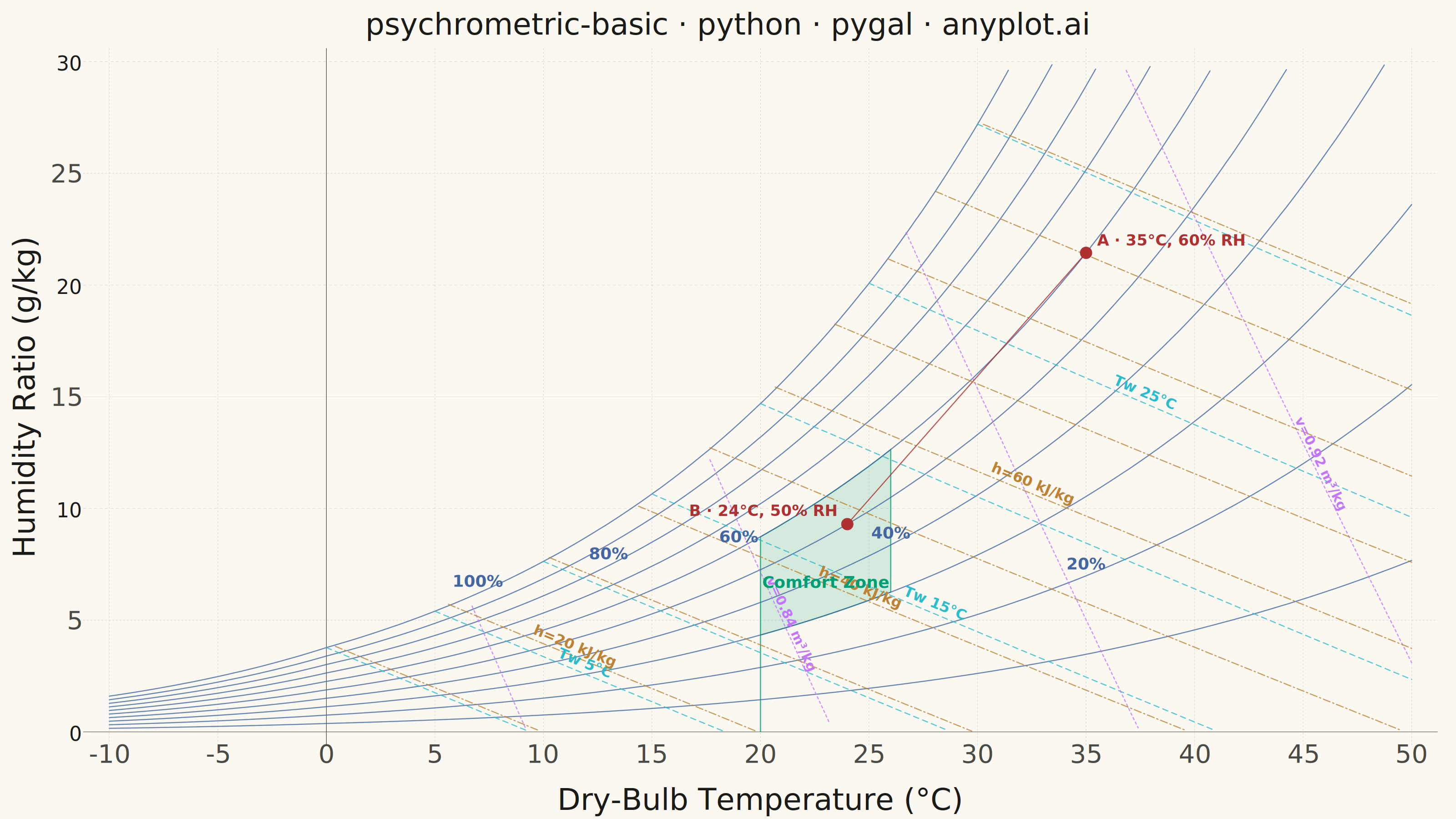
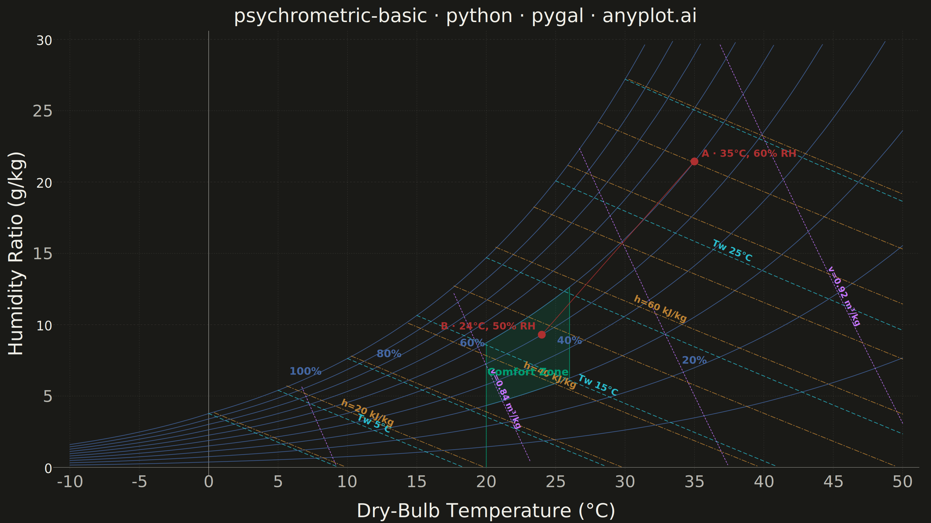
A psychrometric chart plots dry-bulb temperature against humidity ratio, overlaid with curves for relative humidity, wet-bulb temperature, enthalpy, and specific volume. It is the fundamental tool for HVAC system design and air conditioning process analysis. The chart reveals the thermodynamic properties of moist air at a glance, enabling engineers to trace heating, cooling, humidification, and dehumidification processes as paths on the diagram.
""" anyplot.ai
psychrometric-basic: Psychrometric Chart for HVAC
Library: pygal 3.1.0 | Python 3.13.13
Quality: 92/100 | Updated: 2026-06-16
"""

import math
import os

import cairosvg
import numpy as np
import pygal
from pygal.style import Style


# pygal stores its layout (margin_box + coordinate view) in transient state that
# is discarded after render(); keeping it lets us place direct labels at exact
# data coordinates instead of estimating the plot box.
os.environ["PYGAL_KEEP_STATE"] = "1"

# Theme tokens (see prompts/default-style-guide.md "Theme-adaptive Chrome")
THEME = os.getenv("ANYPLOT_THEME", "light")
PAGE_BG = "#FAF8F1" if THEME == "light" else "#1A1A17"
INK = "#1A1A17" if THEME == "light" else "#F0EFE8"
INK_SOFT = "#4A4A44" if THEME == "light" else "#B8B7B0"
INK_MUTED = "#6B6A63" if THEME == "light" else "#A8A79F"
GRID = "rgba(26,26,23,0.15)" if THEME == "light" else "rgba(240,239,232,0.15)"

# Imprint palette — one hue family per psychrometric property type
GREEN = "#009E73"  # comfort zone (good / comfort → green)
BLUE = "#4467A3"  # relative-humidity curves (moisture / water → blue)
CYAN = "#2ABCCD"  # wet-bulb temperature lines
LAV = "#C475FD"  # specific-volume lines
OCHRE = "#BD8233"  # enthalpy lines (energy → warm earth)
RED = "#AE3030"  # HVAC process path (highlighted action)

P_ATM = 101325.0  # Pa — standard sea-level atmosphere

# Data — saturation vapour pressure grid (ASHRAE 2017), vectorised once
t_grid = np.linspace(-15, 55, 1400)
tk = t_grid + 273.15
ln_pws = np.where(
    t_grid >= 0,
    -5.8002206e3 / tk
    + 1.3914993
    - 4.8640239e-2 * tk
    + 4.1764768e-5 * tk**2
    - 1.4452093e-8 * tk**3
    + 6.5459673 * np.log(tk),
    -5.6745359e3 / tk
    + 6.3925247
    - 9.6778430e-3 * tk
    + 6.2215701e-7 * tk**2
    + 2.0747825e-9 * tk**3
    - 9.4840240e-13 * tk**4
    + 4.1635019 * np.log(tk),
)
pws_grid = np.exp(ln_pws)
wsat_grid = 0.62198 * pws_grid / (P_ATM - pws_grid) * 1000  # g/kg at saturation

# Relative-humidity curves (10%–100%)
rh_levels = [1.0, 0.9, 0.8, 0.7, 0.6, 0.5, 0.4, 0.3, 0.2, 0.1]
t_curve = np.linspace(-10, 50, 240)
pws_curve = np.interp(t_curve, t_grid, pws_grid)
rh_curves = {}
for rh in rh_levels:
    pw = rh * pws_curve
    w = 0.62198 * pw / (P_ATM - pw) * 1000
    rh_curves[rh] = [
        (round(float(t), 2), round(float(wi), 3)) for t, wi in zip(t_curve, w, strict=True) if 0 <= wi <= 30
    ]

# Constant wet-bulb lines (ASHRAE psychrometric energy balance, analytical)
wb_temps = [0, 5, 10, 15, 20, 25, 30]
wb_lines = {}
for tw in wb_temps:
    pws_wb = float(np.interp(tw, t_grid, pws_grid))
    w_swb = 0.62198 * pws_wb / (P_ATM - pws_wb)  # kg/kg at saturation
    t_db = np.linspace(tw, 50, 120)
    w = ((2501 - 2.326 * tw) * w_swb - 1.006 * (t_db - tw)) / (2501 + 1.86 * t_db - 4.186 * tw) * 1000
    w_sat = np.interp(t_db, t_grid, wsat_grid)
    wb_lines[tw] = [
        (round(float(t), 2), round(float(wi), 3))
        for t, wi, ws in zip(t_db, w, w_sat, strict=True)
        if 0 <= wi <= min(30, ws + 0.1)
    ]

# Constant enthalpy and specific-volume lines share the dry-bulb sweep
t_line = np.linspace(-10, 50, 220)
wsat_line = np.interp(t_line, t_grid, wsat_grid)

enthalpy_values = [10, 20, 30, 40, 50, 60, 70, 80, 90, 100]
enthalpy_lines = {}
for h in enthalpy_values:
    w = (h - 1.006 * t_line) / (2501 + 1.86 * t_line) * 1000
    enthalpy_lines[h] = [
        (round(float(t), 2), round(float(wi), 3))
        for t, wi, ws in zip(t_line, w, wsat_line, strict=True)
        if 0 <= wi <= min(30, ws + 0.1)
    ]

sv_values = [0.80, 0.84, 0.88, 0.92, 0.96]
sv_lines = {}
for v in sv_values:
    w = (v * P_ATM / 1000 / (0.287042 * (t_line + 273.15)) - 1) / 1.6078 * 1000
    sv_lines[v] = [
        (round(float(t), 2), round(float(wi), 3))
        for t, wi, ws in zip(t_line, w, wsat_line, strict=True)
        if 0 <= wi <= min(30, ws + 0.1)
    ]

# Comfort zone polygon (20–26 °C, 30–60% RH)
ct = np.linspace(20, 26, 30)
pws_c = np.interp(ct, t_grid, pws_grid)
w_low = 0.62198 * (0.30 * pws_c) / (P_ATM - 0.30 * pws_c) * 1000
w_high = 0.62198 * (0.60 * pws_c) / (P_ATM - 0.60 * pws_c) * 1000
comfort_pts = [(round(float(t), 2), round(float(w), 3)) for t, w in zip(ct, w_low, strict=True)]
comfort_pts += [(round(float(t), 2), round(float(w), 3)) for t, w in zip(ct[::-1], w_high[::-1], strict=True)]
comfort_pts.append(comfort_pts[0])

# HVAC process path — cooling & dehumidification (35 °C/60% RH → 24 °C/50% RH)
pa = 0.60 * float(np.interp(35.0, t_grid, pws_grid))
pb = 0.50 * float(np.interp(24.0, t_grid, pws_grid))
state_a = (35.0, round(0.62198 * pa / (P_ATM - pa) * 1000, 3))
state_b = (24.0, round(0.62198 * pb / (P_ATM - pb) * 1000, 3))

# Style — palette assigned per series in add order (comfort first → brand green)
palette = (GREEN,) + (BLUE,) * len(rh_levels) + (CYAN,) * len(wb_temps)
palette += (LAV,) * len(sv_values) + (OCHRE,) * len(enthalpy_values) + (RED,)

custom_style = Style(
    background=PAGE_BG,
    plot_background=PAGE_BG,
    foreground=INK_SOFT,
    foreground_strong=INK,
    foreground_subtle=INK_MUTED,
    opacity="0.95",
    opacity_hover="1",
    colors=palette,
    title_font_size=66,
    label_font_size=56,
    major_label_font_size=44,
    legend_font_size=44,
    value_font_size=36,
    tooltip_font_size=30,
    stroke_width=2.4,
    font_family="Helvetica Neue, Helvetica, Arial, sans-serif",
    guide_stroke_color=GRID,
    major_guide_stroke_color=GRID,
)

chart = pygal.XY(
    width=3200,
    height=1800,
    explicit_size=True,
    style=custom_style,
    title="psychrometric-basic · python · pygal · anyplot.ai",
    x_title="Dry-Bulb Temperature (°C)",
    y_title="Humidity Ratio (g/kg)",
    show_legend=False,
    dots_size=0,
    stroke=True,
    show_x_guides=True,
    show_y_guides=True,
    xrange=(-10, 50),
    range=(0, 30),
    x_labels=list(range(-10, 51, 5)),
    y_labels=list(range(0, 31, 5)),
    print_values=False,
    truncate_label=-1,
    margin_top=30,
    margin_bottom=20,
    margin_left=30,
    margin_right=40,
)

# Comfort zone first → brand green, and drawn beneath every property line
chart.add("Comfort Zone", comfort_pts, show_dots=False, fill=True, stroke_style={"width": 2.4})

# Relative-humidity curves — saturation (100%) thickest and most prominent
for rh in rh_levels:
    width = 6.0 if rh == 1.0 else 2.2
    chart.add(
        f"{int(rh * 100)}% RH",
        rh_curves[rh],
        show_dots=False,
        stroke_style={"width": width, "linecap": "round", "linejoin": "round"},
    )

# Wet-bulb lines — dashed cyan
for tw in wb_temps:
    chart.add(
        f"Tw={tw}°C",
        wb_lines[tw],
        show_dots=False,
        stroke_style={"width": 2.0, "dasharray": "12, 9", "linecap": "round"},
    )

# Specific-volume lines — dotted lavender
for v in sv_values:
    chart.add(
        f"v={v} m³/kg",
        sv_lines[v],
        show_dots=False,
        stroke_style={"width": 2.8, "dasharray": "5, 6", "linecap": "round"},
    )

# Enthalpy lines — dash-dot ochre
for h in enthalpy_values:
    chart.add(
        f"h={h} kJ/kg",
        enthalpy_lines[h],
        show_dots=False,
        stroke_style={"width": 1.8, "dasharray": "16, 6, 3, 6", "linecap": "round"},
    )

# HVAC process path — bold red with state-point markers, on top
chart.add(
    "Cooling & Dehumidification",
    [state_a, state_b],
    show_dots=True,
    dots_size=13,
    stroke_style={"width": 5.0, "linecap": "round"},
)

svg = chart.render(is_unicode=True)

# Soften the comfort-zone fill so it tints rather than masks the RH curves. An inline
# style attribute beats pygal's stylesheet fill-opacity; it targets the only filled
# path (serie-0, the lone `line reactive` class without `nofill`).
svg = svg.replace('class="line reactive"', 'class="line reactive" style="fill-opacity:0.16"', 1)

# Direct labels — exact data→pixel mapping from pygal's own (linear) view transform
ox, oy = chart.margin_box.left, chart.margin_box.top
px_per_t = chart.view.x(1.0) - chart.view.x(0.0)
px_per_w = chart.view.y(1.0) - chart.view.y(0.0)
x_at_0 = ox + chart.view.x(0.0)
y_at_0 = oy + chart.view.y(0.0)

# Pixel coords for each property line, reused for placement and slope
wb_px = {tw: [(x_at_0 + t * px_per_t, y_at_0 + w * px_per_w) for t, w in pts] for tw, pts in wb_lines.items()}
en_px = {h: [(x_at_0 + t * px_per_t, y_at_0 + w * px_per_w) for t, w in pts] for h, pts in enthalpy_lines.items()}
sv_px = {v: [(x_at_0 + t * px_per_t, y_at_0 + w * px_per_w) for t, w in pts] for v, pts in sv_lines.items()}

labels = []

# RH curve labels at staggered temperatures so they ride the curves without piling up
rh_label_t = {1.0: 7, 0.8: 13, 0.6: 19, 0.4: 26, 0.2: 35}
for rh, t_l in rh_label_t.items():
    pws_l = float(np.interp(t_l, t_grid, pws_grid))
    w_l = 0.62198 * (rh * pws_l) / (P_ATM - rh * pws_l) * 1000
    sx = x_at_0 + t_l * px_per_t
    sy = y_at_0 + w_l * px_per_w
    labels.append((sx, sy - 14, f"{int(rh * 100)}%", BLUE, 36, "middle", 0))

# Diagonal family labels — rotated to match each line's local slope
diagonals = [
    (wb_px, [5, 15, 25], 0.50, "Tw {k}°C", CYAN, 32),
    (en_px, [20, 40, 60], 0.40, "h={k} kJ/kg", OCHRE, 32),
    (sv_px, [0.84, 0.92], 0.66, "v={k} m³/kg", LAV, 30),
]
for line_px, keys, frac, template, color, size in diagonals:
    for k in keys:
        pts = line_px[k]
        i = int(len(pts) * frac)
        sx, sy = pts[i]
        x0, y0 = pts[max(0, i - 4)]
        x1, y1 = pts[min(len(pts) - 1, i + 4)]
        ang = math.degrees(math.atan2(y1 - y0, x1 - x0))
        labels.append((sx, sy - 12, template.format(k=k), color, size, "middle", ang))

# Comfort zone, HVAC state points
# Anchored low in the zone (≈37% RH) so it clears the crowded 40%/60% RH band above
cz_pws = float(np.interp(23, t_grid, pws_grid))
cz_w = 0.62198 * (0.37 * cz_pws) / (P_ATM - 0.37 * cz_pws) * 1000
labels.append((x_at_0 + 23 * px_per_t, y_at_0 + cz_w * px_per_w, "Comfort Zone", GREEN, 36, "middle", 0))

ax, ay = x_at_0 + state_a[0] * px_per_t, y_at_0 + state_a[1] * px_per_w
labels.append((ax + 24, ay - 16, "A · 35°C, 60% RH", RED, 34, "start", 0))
bx, by = x_at_0 + state_b[0] * px_per_t, y_at_0 + state_b[1] * px_per_w
labels.append((bx - 24, by - 18, "B · 24°C, 50% RH", RED, 34, "end", 0))

# A thin page-background halo (paint-order stroke) keeps labels legible over lines
label_svg = []
for sx, sy, text, fill, size, anchor, ang in labels:
    transform = f' transform="rotate({ang:.1f},{sx:.1f},{sy:.1f})"' if abs(ang) > 0.5 else ""
    label_svg.append(
        f'<text x="{sx:.1f}" y="{sy:.1f}" font-size="{size}" '
        f'font-family="Helvetica Neue, Helvetica, Arial, sans-serif" font-weight="bold" '
        f'fill="{fill}" stroke="{PAGE_BG}" stroke-width="4" paint-order="stroke" '
        f'text-anchor="{anchor}"{transform}>{text}</text>'
    )

svg = svg.replace("</svg>", "\n".join(label_svg) + "\n</svg>")

# Save — theme-suffixed PNG (gallery) + interactive HTML (pygal is interactive)
with open(f"plot-{THEME}.html", "w", encoding="utf-8") as f:
    f.write(svg)

cairosvg.svg2png(bytestring=svg.encode("utf-8"), write_to=f"plot-{THEME}.png", output_width=3200, output_height=1800)
Runnable source as JSON, for any HTTP client: https://api.anyplot.ai/specs/psychrometric-basic/pygal/code. Any spec id and library id listed in llms-full.txt fit the same URL shape; every URL below is complete and callable.
{
  "spec_id": "psychrometric-basic",
  "language": "python",
  "library": "pygal",
  "page": "https://anyplot.ai/psychrometric-basic/python/pygal",
  "hub": "https://anyplot.ai/psychrometric-basic",
  "code_json": "https://api.anyplot.ai/specs/psychrometric-basic/pygal/code",
  "spec_json": "https://api.anyplot.ai/specs/psychrometric-basic",
  "render_light_png": "https://storage.googleapis.com/anyplot-images/plots/psychrometric-basic/python/pygal/plot-light.png",
  "render_dark_png": "https://storage.googleapis.com/anyplot-images/plots/psychrometric-basic/python/pygal/plot-dark.png",
  "interactive_light_html": "https://storage.googleapis.com/anyplot-images/plots/psychrometric-basic/python/pygal/plot-light.html",
  "interactive_dark_html": "https://storage.googleapis.com/anyplot-images/plots/psychrometric-basic/python/pygal/plot-dark.html",
  "quality_score": 92.0,
  "license": "MIT",
  "guide": "https://anyplot.ai/llms.txt"
}
Part of Psychrometric Chart for HVAC on anyplot.ai.