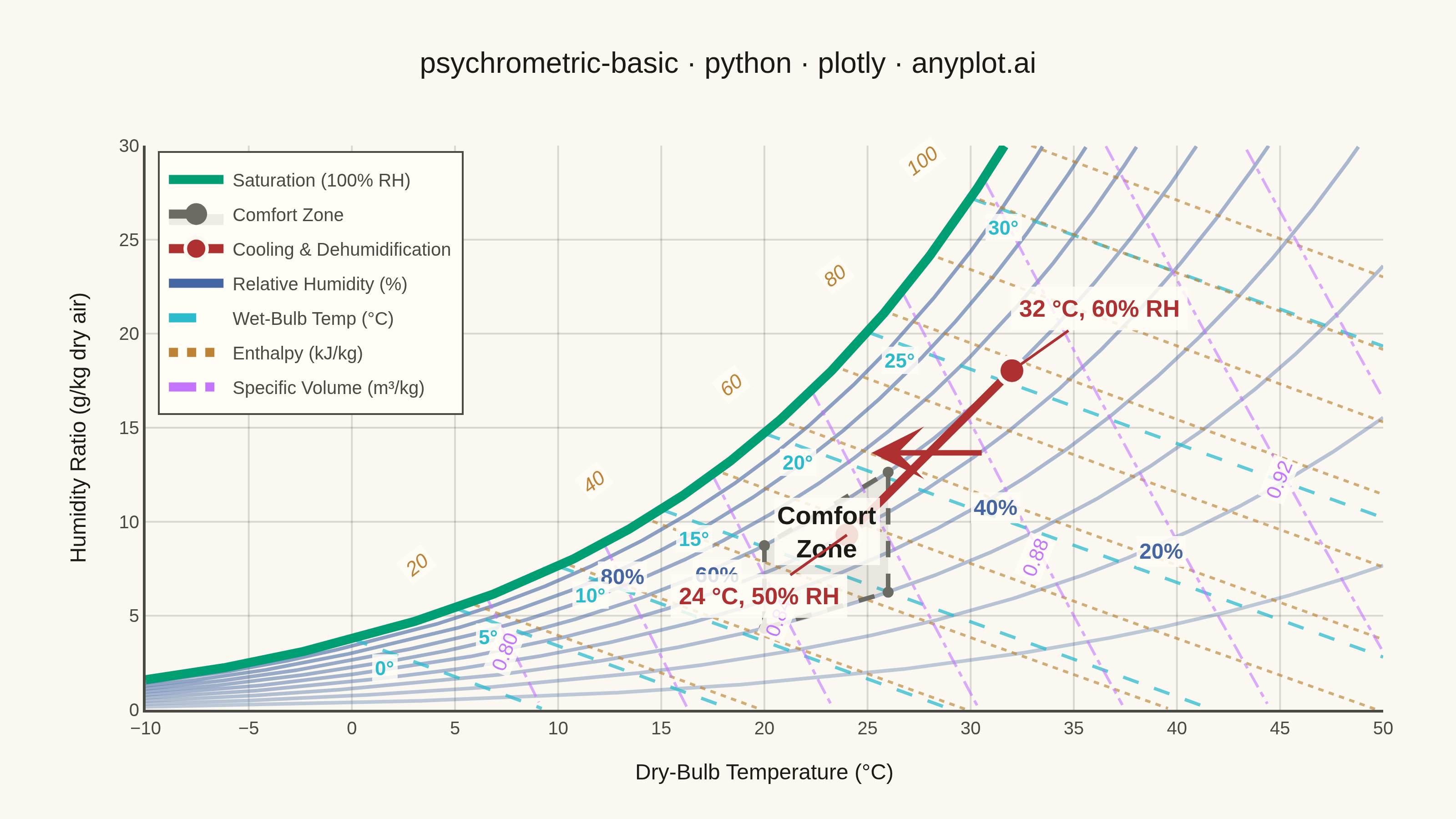
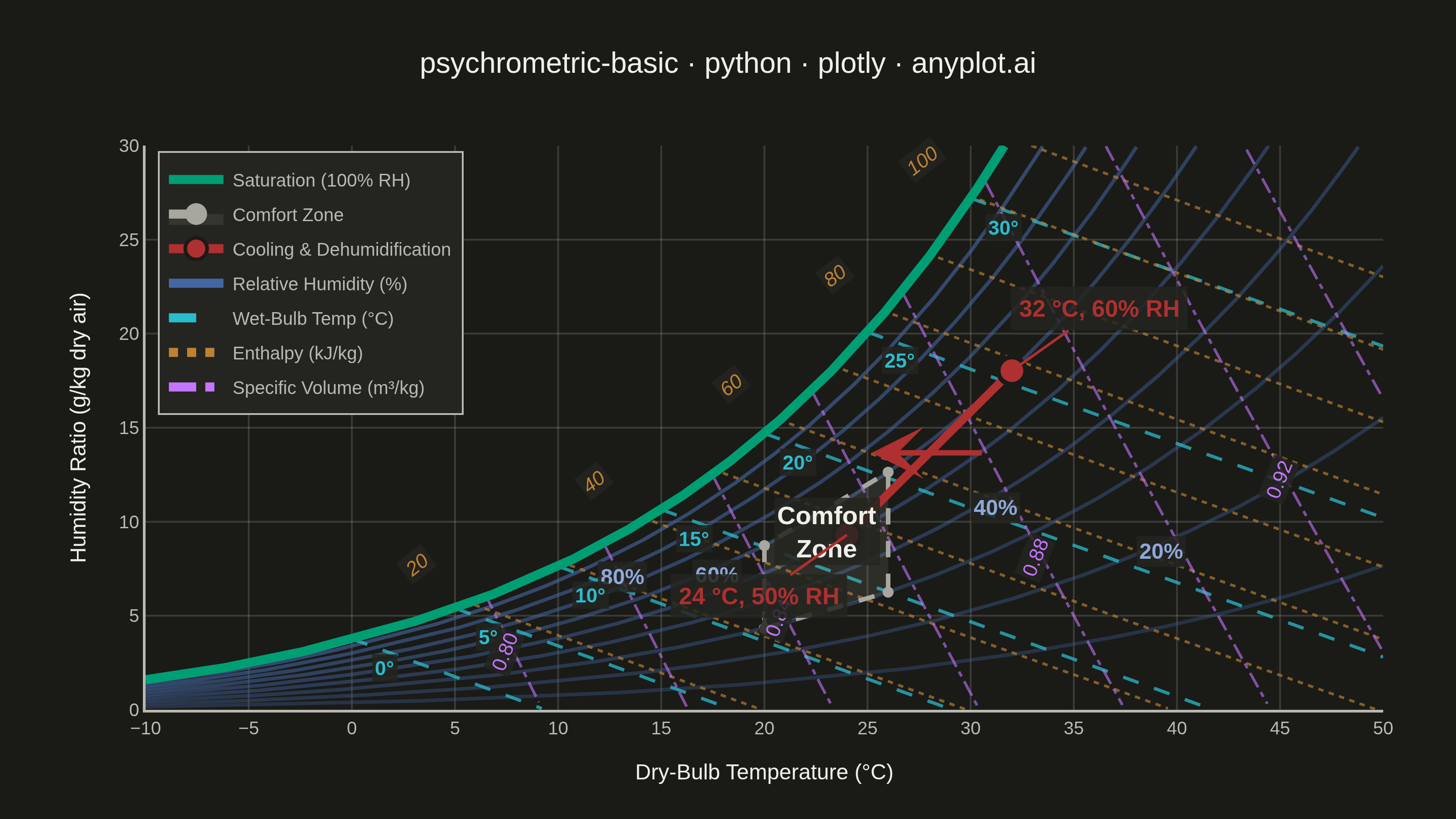
A psychrometric chart plots dry-bulb temperature against humidity ratio, overlaid with curves for relative humidity, wet-bulb temperature, enthalpy, and specific volume. It is the fundamental tool for HVAC system design and air conditioning process analysis. The chart reveals the thermodynamic properties of moist air at a glance, enabling engineers to trace heating, cooling, humidification, and dehumidification processes as paths on the diagram.
""" anyplot.ai
psychrometric-basic: Psychrometric Chart for HVAC
Library: plotly 6.8.0 | Python 3.13.13
Quality: 92/100 | Updated: 2026-06-16
"""

import os

import numpy as np
import plotly.graph_objects as go


# Theme-adaptive chrome (see prompts/default-style-guide.md "Theme-adaptive Chrome")
THEME = os.getenv("ANYPLOT_THEME", "light")
PAGE_BG = "#FAF8F1" if THEME == "light" else "#1A1A17"
ELEVATED_BG = "#FFFDF6" if THEME == "light" else "#242420"
INK = "#1A1A17" if THEME == "light" else "#F0EFE8"
INK_SOFT = "#4A4A44" if THEME == "light" else "#B8B7B0"
GRID = "rgba(26,26,23,0.15)" if THEME == "light" else "rgba(240,239,232,0.15)"
LABEL_BG = "rgba(255,253,246,0.85)" if THEME == "light" else "rgba(36,36,32,0.85)"

# Imprint palette — one hue family per psychrometric property (theme-independent)
SAT = "#009E73"  # brand green — saturation curve (ALWAYS first series)
RH = (68, 103, 163)  # #4467A3 blue — relative-humidity curves
# RH *labels* get a brighter blue in dark theme so they read as crisply as the
# cyan/ochre labels against the near-black surface (curve color stays identical).
RH_LABEL = RH if THEME == "light" else (143, 168, 218)  # #8FA8DA
WB = (42, 188, 205)  # #2ABCCD cyan — wet-bulb lines
ENTH = (189, 130, 51)  # #BD8233 ochre — enthalpy lines
VOL = (196, 117, 253)  # #C475FD lavender — specific-volume lines
PROC = "#AE3030"  # matte red — highlighted HVAC process (semantic emphasis)
COMFORT = "#6B6A63" if THEME == "light" else "#A8A79F"  # muted neutral — context region

# Standard sea-level atmosphere
P_ATM = 101325  # Pa

# Saturation pressure over a fine dry-bulb grid (ASHRAE 2017 Ch.1) — computed ONCE,
# then np.interp reuses it everywhere instead of re-deriving the formula per loop.
t_fine = np.linspace(-10, 50, 1200)
t_k = t_fine + 273.15
p_ws_fine = np.where(
    t_fine >= 0,
    np.exp(
        -5800.2206 / t_k
        + 1.3914993
        - 0.048640239 * t_k
        + 0.000041764768 * t_k**2
        - 0.000000014452093 * t_k**3
        + 6.5459673 * np.log(t_k)
    ),
    np.exp(
        -5674.5359 / t_k
        + 6.3925247
        - 0.009677843 * t_k
        + 0.00000062215701 * t_k**2
        + 2.0747825e-09 * t_k**3
        - 9.484024e-13 * t_k**4
        + 4.1635019 * np.log(t_k)
    ),
)
w_sat_fine = 0.621945 * p_ws_fine / (P_ATM - p_ws_fine) * 1000  # g/kg

W_MAX = 30.0  # y-axis ceiling
fig = go.Figure()

# --- Relative-humidity curves (10%-90%) — graduated opacity, drawn under saturation ---
# Anchor fractions chosen so RH labels fan into open pockets, clear of the
# central process path / comfort-zone / specific-volume labels (see VQ-02).
rh_label_frac = {20: 0.80, 40: 0.68, 60: 0.52, 80: 0.48}
for rh_pct in range(10, 100, 10):
    p_w = (rh_pct / 100.0) * p_ws_fine
    w = 0.621945 * p_w / (P_ATM - p_w) * 1000
    mask = (w >= 0) & (w <= W_MAX)
    t_plot, w_plot = t_fine[mask], w[mask]
    h_vals = 1.006 * t_plot + (w_plot / 1000) * (2501 + 1.86 * t_plot)
    alpha = 0.30 + rh_pct * 0.0035
    fig.add_trace(
        go.Scatter(
            x=t_plot,
            y=w_plot,
            mode="lines",
            line={"color": f"rgba({RH[0]},{RH[1]},{RH[2]},{alpha:.2f})", "width": 2.0},
            showlegend=False,
            customdata=np.column_stack([h_vals, np.full_like(t_plot, rh_pct)]),
            hovertemplate=(
                "<b>%{customdata[1]:.0f}% RH</b><br>"
                "Dry-Bulb: %{x:.1f} °C<br>"
                "Humidity Ratio: %{y:.2f} g/kg<br>"
                "Enthalpy: %{customdata[0]:.1f} kJ/kg<extra></extra>"
            ),
        )
    )
    if rh_pct in rh_label_frac and len(t_plot) > 20:
        idx = int(len(t_plot) * rh_label_frac[rh_pct])
        fig.add_annotation(
            x=float(t_plot[idx]),
            y=float(w_plot[idx]),
            text=f"<b>{rh_pct}%</b>",
            showarrow=False,
            font={"size": 12, "color": f"rgb({RH_LABEL[0]},{RH_LABEL[1]},{RH_LABEL[2]})"},
            xshift=14,
            yshift=2,
            bgcolor=LABEL_BG,
        )

# --- Wet-bulb temperature lines (constant t_wb, labeled near the saturation end) ---
for t_wb in range(0, 35, 5):
    t_arr = np.linspace(t_wb, 50, 240)
    p_ws_wb = float(np.interp(t_wb, t_fine, p_ws_fine))
    w_s_wb = 0.621945 * p_ws_wb / (P_ATM - p_ws_wb)
    w = (w_s_wb - 1.006 * (t_arr - t_wb) / (2501 + 1.86 * t_wb)) * 1000
    w_lid = np.interp(t_arr, t_fine, w_sat_fine)
    mask = (w >= 0) & (w <= W_MAX) & (w <= w_lid + 0.3)
    t_plot, w_plot = t_arr[mask], w[mask]
    if len(t_plot) > 5:
        fig.add_trace(
            go.Scatter(
                x=t_plot,
                y=w_plot,
                mode="lines",
                line={"color": f"rgba({WB[0]},{WB[1]},{WB[2]},0.75)", "width": 1.8, "dash": "dash"},
                showlegend=False,
                hovertemplate=(
                    f"<b>Wet-Bulb: {t_wb} °C</b><br>"
                    "Dry-Bulb: %{x:.1f} °C<br>"
                    "Humidity Ratio: %{y:.2f} g/kg<extra></extra>"
                ),
            )
        )
        # Wet-bulb labels nudge DOWN-RIGHT (into the chart, below the saturation
        # curve) while enthalpy labels go UP-LEFT — the two families converge on
        # the curve, so opposite offsets keep their labels from stacking (VQ-02).
        fig.add_annotation(
            x=float(t_plot[0]),
            y=float(w_plot[0]),
            text=f"<b>{t_wb}°</b>",
            showarrow=False,
            font={"size": 11, "color": f"rgb({WB[0]},{WB[1]},{WB[2]})"},
            xshift=18,
            yshift=-16,
            bgcolor=LABEL_BG,
        )

# --- Constant-enthalpy lines (kJ/kg), labeled at the upper-left saturation end ---
for h in range(20, 120, 10):
    t_arr = np.linspace(-10, 50, 300)
    w = (h - 1.006 * t_arr) / (2501 + 1.86 * t_arr) * 1000
    w_lid = np.interp(t_arr, t_fine, w_sat_fine)
    mask = (w >= 0) & (w <= W_MAX) & (w <= w_lid + 0.3)
    t_plot, w_plot = t_arr[mask], w[mask]
    if len(t_plot) > 5:
        fig.add_trace(
            go.Scatter(
                x=t_plot,
                y=w_plot,
                mode="lines",
                line={"color": f"rgba({ENTH[0]},{ENTH[1]},{ENTH[2]},0.65)", "width": 1.5, "dash": "dot"},
                showlegend=False,
                hovertemplate=(
                    f"<b>Enthalpy: {h} kJ/kg</b><br>"
                    "Dry-Bulb: %{x:.1f} °C<br>"
                    "Humidity Ratio: %{y:.2f} g/kg<extra></extra>"
                ),
            )
        )
        if h % 20 == 0:
            fig.add_annotation(
                x=float(t_plot[0]),
                y=float(w_plot[0]),
                text=f"<i>{h}</i>",
                showarrow=False,
                font={"size": 11, "color": f"rgb({ENTH[0]},{ENTH[1]},{ENTH[2]})"},
                xshift=-26,
                yshift=20,
                bgcolor=LABEL_BG,
                textangle=-38,
            )

# --- Constant specific-volume lines (m³/kg dry air) ---
for v_100 in range(80, 96, 2):
    v = v_100 / 100.0
    t_arr = np.linspace(-10, 50, 300)
    w = (P_ATM * v / (287.042 * (t_arr + 273.15)) - 1) / (1 + 287.042 / 461.524) * 1000
    w_lid = np.interp(t_arr, t_fine, w_sat_fine)
    mask = (w >= 0) & (w <= W_MAX) & (w <= w_lid + 0.3)
    t_plot, w_plot = t_arr[mask], w[mask]
    if len(t_plot) > 5:
        fig.add_trace(
            go.Scatter(
                x=t_plot,
                y=w_plot,
                mode="lines",
                line={"color": f"rgba({VOL[0]},{VOL[1]},{VOL[2]},0.60)", "width": 1.5, "dash": "dashdot"},
                showlegend=False,
                hovertemplate=(
                    f"<b>Specific Volume: {v:.2f} m³/kg</b><br>"
                    "Dry-Bulb: %{x:.1f} °C<br>"
                    "Humidity Ratio: %{y:.2f} g/kg<extra></extra>"
                ),
            )
        )
        if v_100 % 4 == 0:
            # Label lower-right along each line so '0.84' clears the central
            # comfort-zone / process annotations rather than sitting on them.
            idx = int(len(t_plot) * 0.68)
            fig.add_annotation(
                x=float(t_plot[idx]),
                y=float(w_plot[idx]),
                text=f"{v:.2f}",
                showarrow=False,
                font={"size": 11, "color": f"rgb({VOL[0]},{VOL[1]},{VOL[2]})"},
                xshift=-10,
                yshift=10,
                bgcolor=LABEL_BG,
                textangle=-68,
            )

# --- Saturation curve (100% RH) — prominent upper boundary, drawn on top ---
mask_sat = w_sat_fine <= W_MAX
t_sat, w_sat = t_fine[mask_sat], w_sat_fine[mask_sat]
h_sat = 1.006 * t_sat + (w_sat / 1000) * (2501 + 1.86 * t_sat)
fig.add_trace(
    go.Scatter(
        x=t_sat,
        y=w_sat,
        mode="lines",
        line={"color": SAT, "width": 5},
        name="Saturation (100% RH)",
        customdata=np.column_stack([h_sat]),
        hovertemplate=(
            "<b>Saturation Curve</b><br>"
            "Dry-Bulb: %{x:.1f} °C<br>"
            "Humidity Ratio: %{y:.2f} g/kg<br>"
            "Enthalpy: %{customdata[0]:.1f} kJ/kg<extra></extra>"
        ),
    )
)

# --- Comfort zone (ASHRAE: 20-26 °C, 30-60% RH) ---
ct = np.array([20.0, 26.0, 26.0, 20.0])
crh = np.array([0.30, 0.30, 0.60, 0.60])
p_ws_c = np.interp(ct, t_fine, p_ws_fine)
cw = 0.621945 * (crh * p_ws_c) / (P_ATM - crh * p_ws_c) * 1000
fig.add_trace(
    go.Scatter(
        x=np.append(ct, ct[0]),
        y=np.append(cw, cw[0]),
        fill="toself",
        fillcolor="rgba(107,106,99,0.12)" if THEME == "light" else "rgba(168,167,159,0.14)",
        line={"color": COMFORT, "width": 2.5, "dash": "dash"},
        name="Comfort Zone",
        hovertemplate="<b>ASHRAE Comfort Zone</b><br>20–26 °C, 30–60% RH<extra></extra>",
    )
)
fig.add_annotation(
    x=23,
    y=float((cw[1] + cw[2]) / 2),
    text="<b>Comfort<br>Zone</b>",
    showarrow=False,
    font={"size": 14, "color": INK},
    bgcolor=LABEL_BG,
)

# --- HVAC process path: cooling & dehumidification (32 °C/60% RH → 24 °C/50% RH) ---
st_t = np.array([32.0, 24.0])
st_rh = np.array([0.60, 0.50])
p_ws_s = np.interp(st_t, t_fine, p_ws_fine)
st_w = 0.621945 * (st_rh * p_ws_s) / (P_ATM - st_rh * p_ws_s) * 1000
st_h = 1.006 * st_t + (st_w / 1000) * (2501 + 1.86 * st_t)
fig.add_trace(
    go.Scatter(
        x=st_t,
        y=st_w,
        mode="lines+markers",
        line={"color": PROC, "width": 4.5},
        marker={"size": 15, "color": PROC, "line": {"color": PAGE_BG, "width": 2.5}},
        name="Cooling & Dehumidification",
        customdata=np.column_stack([st_rh * 100, st_h]),
        hovertemplate=(
            "<b>State Point</b><br>"
            "Dry-Bulb: %{x:.0f} °C<br>"
            "RH: %{customdata[0]:.0f}%<br>"
            "Humidity Ratio: %{y:.1f} g/kg<br>"
            "Enthalpy: %{customdata[1]:.1f} kJ/kg<extra></extra>"
        ),
    )
)
fig.add_annotation(
    x=float(st_t[1] + 1.2),
    y=float((st_w[0] + st_w[1]) / 2),
    ax=float(st_t[0] - 1.2),
    ay=float((st_w[0] + st_w[1]) / 2),
    xref="x",
    yref="y",
    axref="x",
    ayref="y",
    showarrow=True,
    arrowhead=3,
    arrowsize=1.6,
    arrowwidth=3,
    arrowcolor=PROC,
)
fig.add_annotation(
    x=float(st_t[0]),
    y=float(st_w[0]),
    text="<b>32 °C, 60% RH</b>",
    showarrow=True,
    arrowhead=0,
    arrowwidth=1.5,
    arrowcolor=PROC,
    ax=48,
    ay=-34,
    font={"size": 13, "color": PROC},
    bgcolor=LABEL_BG,
    borderpad=4,
)
fig.add_annotation(
    x=float(st_t[1]),
    y=float(st_w[1]),
    text="<b>24 °C, 50% RH</b>",
    showarrow=True,
    arrowhead=0,
    arrowwidth=1.5,
    arrowcolor=PROC,
    ax=-48,
    ay=34,
    font={"size": 13, "color": PROC},
    bgcolor=LABEL_BG,
    borderpad=4,
)

# --- Legend proxies for the unlabeled property families ---
for lname, lrgb, ldash in [
    ("Relative Humidity (%)", RH, "solid"),
    ("Wet-Bulb Temp (°C)", WB, "dash"),
    ("Enthalpy (kJ/kg)", ENTH, "dot"),
    ("Specific Volume (m³/kg)", VOL, "dashdot"),
]:
    fig.add_trace(
        go.Scatter(
            x=[None],
            y=[None],
            mode="lines",
            line={"color": f"rgb({lrgb[0]},{lrgb[1]},{lrgb[2]})", "width": 2.5, "dash": ldash},
            name=lname,
        )
    )

# --- Layout ---
axis_common = {
    "tickfont": {"size": 10, "color": INK_SOFT},
    "dtick": 5,
    "gridcolor": GRID,
    "gridwidth": 1,
    "zeroline": False,
    "showline": True,
    "linewidth": 1.5,
    "linecolor": INK_SOFT,
}
fig.update_layout(
    autosize=False,
    title={
        "text": "psychrometric-basic · python · plotly · anyplot.ai",
        "font": {"size": 16, "color": INK},
        "x": 0.5,
        "xanchor": "center",
    },
    paper_bgcolor=PAGE_BG,
    plot_bgcolor=PAGE_BG,
    font={"color": INK},
    xaxis={
        "title": {"text": "Dry-Bulb Temperature (°C)", "font": {"size": 12, "color": INK}},
        "range": [-10, 50],
        **axis_common,
    },
    yaxis={
        "title": {"text": "Humidity Ratio (g/kg dry air)", "font": {"size": 12, "color": INK}},
        "range": [0, W_MAX],
        **axis_common,
    },
    legend={
        "font": {"size": 10, "color": INK_SOFT},
        "x": 0.01,
        "y": 0.99,
        "xanchor": "left",
        "yanchor": "top",
        "bgcolor": ELEVATED_BG,
        "bordercolor": INK_SOFT,
        "borderwidth": 1,
        "itemsizing": "constant",
    },
    margin={"l": 80, "r": 40, "t": 80, "b": 60},
    hoverlabel={"bgcolor": ELEVATED_BG, "font": {"size": 13, "color": INK}, "bordercolor": INK_SOFT},
    hovermode="closest",
)

# Save
fig.write_image(f"plot-{THEME}.png", width=800, height=450, scale=4)
fig.write_html(f"plot-{THEME}.html", include_plotlyjs="cdn")
Runnable source as JSON, for any HTTP client: https://api.anyplot.ai/specs/psychrometric-basic/plotly/code. Any spec id and library id listed in llms-full.txt fit the same URL shape; every URL below is complete and callable.
{
  "spec_id": "psychrometric-basic",
  "language": "python",
  "library": "plotly",
  "page": "https://anyplot.ai/psychrometric-basic/python/plotly",
  "hub": "https://anyplot.ai/psychrometric-basic",
  "code_json": "https://api.anyplot.ai/specs/psychrometric-basic/plotly/code",
  "spec_json": "https://api.anyplot.ai/specs/psychrometric-basic",
  "render_light_png": "https://storage.googleapis.com/anyplot-images/plots/psychrometric-basic/python/plotly/plot-light.png",
  "render_dark_png": "https://storage.googleapis.com/anyplot-images/plots/psychrometric-basic/python/plotly/plot-dark.png",
  "interactive_light_html": "https://storage.googleapis.com/anyplot-images/plots/psychrometric-basic/python/plotly/plot-light.html",
  "interactive_dark_html": "https://storage.googleapis.com/anyplot-images/plots/psychrometric-basic/python/plotly/plot-dark.html",
  "quality_score": 92.0,
  "license": "MIT",
  "guide": "https://anyplot.ai/llms.txt"
}
Part of Psychrometric Chart for HVAC on anyplot.ai.