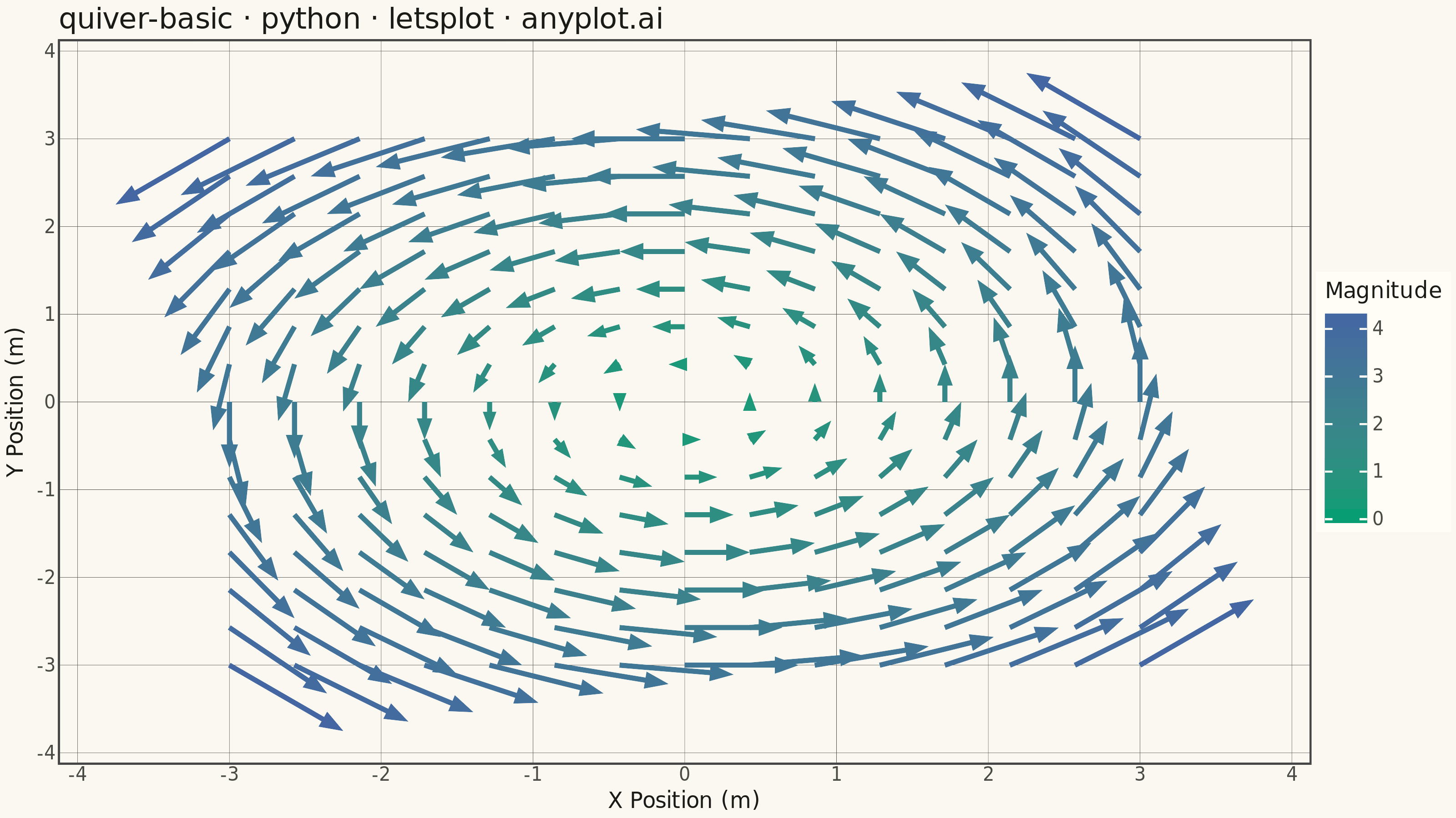
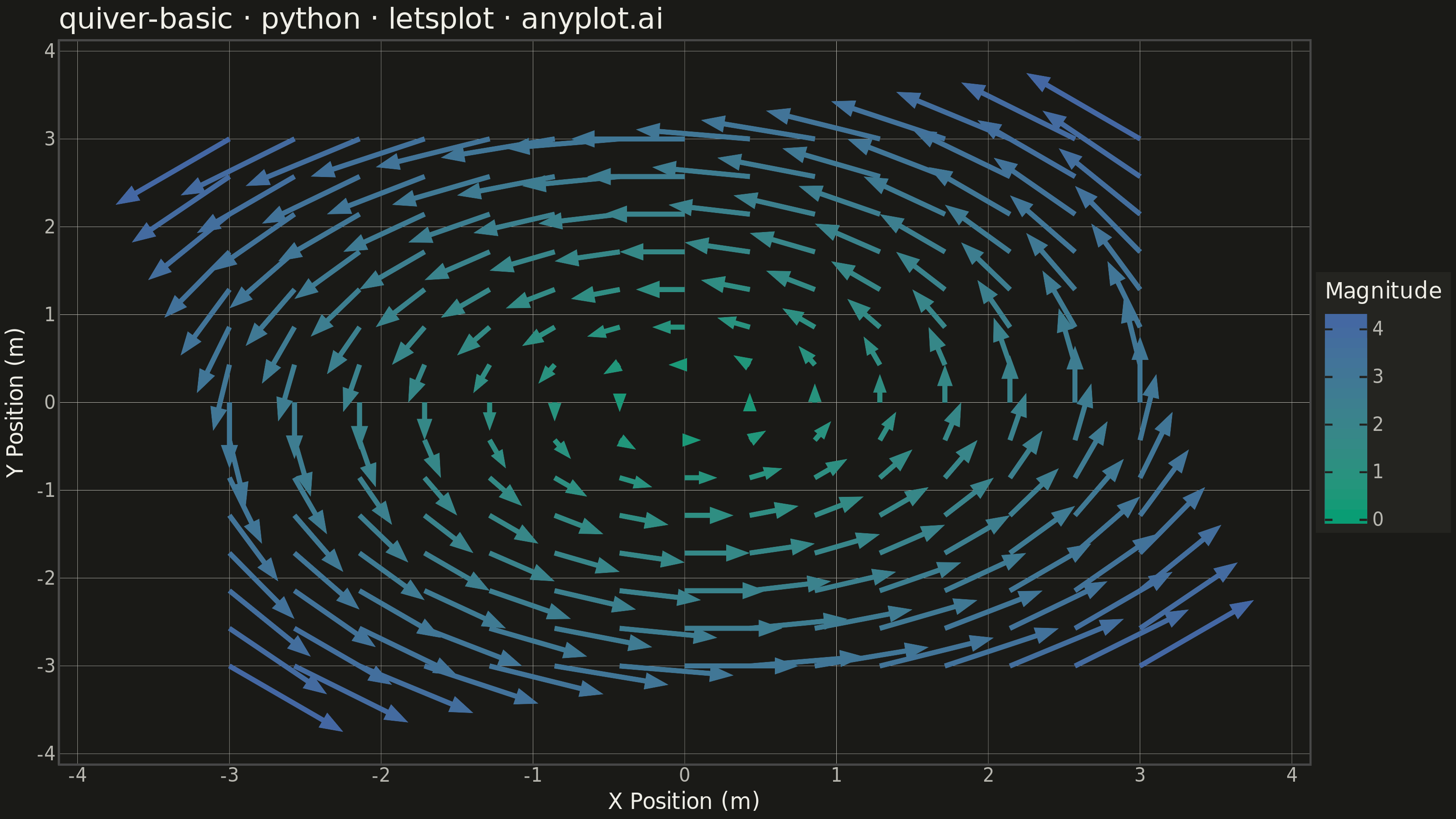
A quiver plot displays vector fields using arrows positioned at grid points. Each arrow represents a vector at that location, with direction indicating the vector's angle and length proportional to its magnitude. This visualization reveals flow patterns, gradients, and field structure in two-dimensional data.
""" anyplot.ai
quiver-basic: Basic Quiver Plot
Library: letsplot 4.11.0 | Python 3.13.14
Quality: 88/100 | Updated: 2026-07-24
"""

import os

import numpy as np
import pandas as pd
from lets_plot import (
    LetsPlot,
    aes,
    arrow,
    element_blank,
    element_line,
    element_rect,
    element_text,
    geom_segment,
    ggplot,
    ggsize,
    labs,
    layer_tooltips,
    scale_color_gradient,
    theme,
    theme_minimal,
)
from lets_plot.export import ggsave


LetsPlot.setup_html()

# Theme tokens
THEME = os.getenv("ANYPLOT_THEME", "light")
PAGE_BG = "#FAF8F1" if THEME == "light" else "#1A1A17"
ELEVATED_BG = "#FFFDF6" if THEME == "light" else "#242420"
INK = "#1A1A17" if THEME == "light" else "#F0EFE8"
INK_SOFT = "#4A4A44" if THEME == "light" else "#B8B7B0"

# Data - 2D rotation vector field: u = -y, v = x (circular flow pattern)
grid_size = 15
x_range = np.linspace(-3, 3, grid_size)
y_range = np.linspace(-3, 3, grid_size)
X, Y = np.meshgrid(x_range, y_range)
X = X.flatten()
Y = Y.flatten()

# Vector components (rotation field: u = -y, v = x)
U = -Y
V = X

magnitude = np.sqrt(U**2 + V**2)

# Grid spacing is 6/(grid_size-1) ~= 0.43; scale_factor keeps the longest
# scaled arrow (at the outer ring, magnitude ~4.24) shorter than that
# spacing so shafts/heads stay visually separated.
scale_factor = 0.08
U_scaled = U * scale_factor
V_scaled = V * scale_factor

df = pd.DataFrame({"x": X, "y": Y, "xend": X + U_scaled, "yend": Y + V_scaled, "magnitude": magnitude, "u": U, "v": V})

# Theme-adaptive chrome
anyplot_theme = theme(
    plot_background=element_rect(fill=PAGE_BG, color=PAGE_BG),
    panel_background=element_rect(fill=PAGE_BG),
    panel_grid_major=element_line(color=INK_SOFT, size=0.15),
    panel_grid_minor=element_blank(),
    axis_title=element_text(color=INK, size=12),
    axis_text=element_text(color=INK_SOFT, size=10),
    axis_line=element_line(color=INK_SOFT),
    plot_title=element_text(color=INK, size=16),
    legend_background=element_rect(fill=ELEVATED_BG, color=INK_SOFT),
    legend_text=element_text(color=INK_SOFT, size=10),
    legend_title=element_text(color=INK, size=12),
)

# Plot — magnitude is single-polarity (>= 0), so the Imprint sequential gradient applies
segment_tooltips = layer_tooltips().line("Position|(@x, @y)").line("u, v|(@u, @v)").line("Magnitude|@magnitude")

plot = (
    ggplot(df, aes(x="x", y="y", xend="xend", yend="yend", color="magnitude"))
    + geom_segment(arrow=arrow(angle=20, length=8, type="closed"), size=1.2, tooltips=segment_tooltips)
    + scale_color_gradient(low="#009E73", high="#4467A3", name="Magnitude")
    + labs(x="X Position (m)", y="Y Position (m)", title="quiver-basic · python · letsplot · anyplot.ai")
    + ggsize(800, 450)
    + theme_minimal()
    + anyplot_theme
)

# Save PNG (scale 4x to get 3200 x 1800 px) and HTML
ggsave(plot, filename=f"plot-{THEME}.png", path=".", scale=4)
ggsave(plot, filename=f"plot-{THEME}.html", path=".")
Runnable source as JSON, for any HTTP client: https://api.anyplot.ai/specs/quiver-basic/letsplot/code. Any spec id and library id listed in llms-full.txt fit the same URL shape; every URL below is complete and callable.
{
  "spec_id": "quiver-basic",
  "language": "python",
  "library": "letsplot",
  "page": "https://anyplot.ai/quiver-basic/python/letsplot",
  "hub": "https://anyplot.ai/quiver-basic",
  "code_json": "https://api.anyplot.ai/specs/quiver-basic/letsplot/code",
  "spec_json": "https://api.anyplot.ai/specs/quiver-basic",
  "render_light_png": "https://storage.googleapis.com/anyplot-images/plots/quiver-basic/python/letsplot/plot-light.png",
  "render_dark_png": "https://storage.googleapis.com/anyplot-images/plots/quiver-basic/python/letsplot/plot-dark.png",
  "interactive_light_html": "https://storage.googleapis.com/anyplot-images/plots/quiver-basic/python/letsplot/plot-light.html",
  "interactive_dark_html": "https://storage.googleapis.com/anyplot-images/plots/quiver-basic/python/letsplot/plot-dark.html",
  "quality_score": 88.0,
  "license": "MIT",
  "guide": "https://anyplot.ai/llms.txt"
}
Part of Basic Quiver Plot on anyplot.ai.