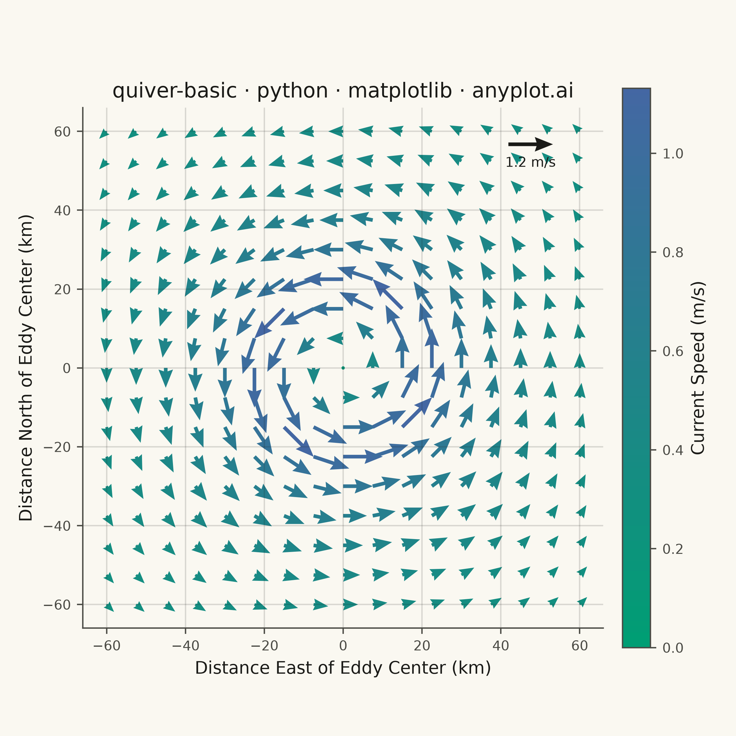
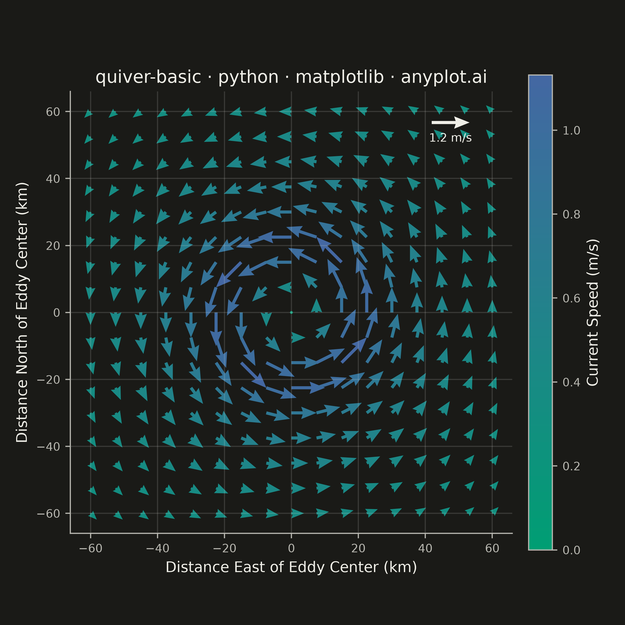
A quiver plot displays vector fields using arrows positioned at grid points. Each arrow represents a vector at that location, with direction indicating the vector's angle and length proportional to its magnitude. This visualization reveals flow patterns, gradients, and field structure in two-dimensional data.
""" anyplot.ai
quiver-basic: Basic Quiver Plot
Library: matplotlib 3.11.1 | Python 3.13.14
Quality: 90/100 | Updated: 2026-07-24
"""

import os
import sys


# Prevent this file (matplotlib.py) from shadowing the real matplotlib package
sys.path = [p for p in sys.path if os.path.abspath(p or ".") != os.path.dirname(os.path.abspath(__file__))]

import matplotlib.pyplot as plt
import numpy as np
from matplotlib.colors import LinearSegmentedColormap


# Theme tokens
THEME = os.getenv("ANYPLOT_THEME", "light")
PAGE_BG = "#FAF8F1" if THEME == "light" else "#1A1A17"
INK = "#1A1A17" if THEME == "light" else "#F0EFE8"
INK_SOFT = "#4A4A44" if THEME == "light" else "#B8B7B0"

# Imprint sequential colormap (brand green -> blue) for single-polarity speed
imprint_seq = LinearSegmentedColormap.from_list("imprint_seq", ["#009E73", "#4467A3"])

# Data - Rankine combined vortex, a textbook model for an ocean mesoscale eddy:
# solid-body rotation inside the core radius, irrotational 1/r decay outside.
# This keeps arrows near the center visible (unlike a pure u=-y, v=x field,
# whose magnitude vanishes to zero exactly at the origin) while still tapering
# gently at the domain edges.
grid_size = 17
km = np.linspace(-60, 60, grid_size)
X, Y = np.meshgrid(km, km)
R = np.sqrt(X**2 + Y**2)
theta = np.arctan2(Y, X)

core_radius = 20.0  # km, radius of peak tangential speed
v_max = 1.2  # m/s, peak tangential current speed at the core edge
R_safe = np.where(R == 0, 1e-6, R)
speed = np.where(R <= core_radius, v_max * R / core_radius, v_max * core_radius / R_safe)

U = -speed * np.sin(theta)
V = speed * np.cos(theta)

# Plot
fig, ax = plt.subplots(figsize=(6, 6), dpi=400, facecolor=PAGE_BG)
ax.set_facecolor(PAGE_BG)

quiver = ax.quiver(
    X, Y, U, V, speed, cmap=imprint_seq, scale=14, width=0.007, headwidth=4, headlength=5, headaxislength=4.5
)

# Reference arrow — a distinctly matplotlib feature that anchors the eye to
# an exact speed, since color alone only conveys relative magnitude.
ax.quiverkey(
    quiver,
    X=0.86,
    Y=0.93,
    U=v_max,
    label=f"{v_max:.1f} m/s",
    labelpos="S",
    coordinates="axes",
    color=INK,
    labelcolor=INK,
    fontproperties={"size": 8},
)

# Colorbar
cbar = plt.colorbar(quiver, ax=ax, shrink=0.8, pad=0.03)
cbar.set_label("Current Speed (m/s)", fontsize=10, color=INK)
cbar.ax.tick_params(labelsize=8, colors=INK_SOFT)
cbar.ax.set_facecolor(PAGE_BG)
cbar.outline.set_edgecolor(INK_SOFT)

# Style
title = "quiver-basic · python · matplotlib · anyplot.ai"
n = len(title)
ratio = 67 / n if n > 67 else 1.0
title_fontsize = max(8, round(12 * ratio))

ax.set_xlabel("Distance East of Eddy Center (km)", fontsize=10, color=INK)
ax.set_ylabel("Distance North of Eddy Center (km)", fontsize=10, color=INK)
ax.set_title(title, fontsize=title_fontsize, fontweight="medium", color=INK)
ax.tick_params(axis="both", labelsize=8, colors=INK_SOFT)
ax.set_aspect("equal")

ax.spines["top"].set_visible(False)
ax.spines["right"].set_visible(False)
for s in ("left", "bottom"):
    ax.spines[s].set_color(INK_SOFT)

ax.grid(True, alpha=0.15, linewidth=0.8, color=INK)

fig.tight_layout()
plt.savefig(f"plot-{THEME}.png", dpi=400, facecolor=PAGE_BG)  # do NOT add bbox_inches='tight'
Runnable source as JSON, for any HTTP client: https://api.anyplot.ai/specs/quiver-basic/matplotlib/code. Any spec id and library id listed in llms-full.txt fit the same URL shape; every URL below is complete and callable.
{
  "spec_id": "quiver-basic",
  "language": "python",
  "library": "matplotlib",
  "page": "https://anyplot.ai/quiver-basic/python/matplotlib",
  "hub": "https://anyplot.ai/quiver-basic",
  "code_json": "https://api.anyplot.ai/specs/quiver-basic/matplotlib/code",
  "spec_json": "https://api.anyplot.ai/specs/quiver-basic",
  "render_light_png": "https://storage.googleapis.com/anyplot-images/plots/quiver-basic/python/matplotlib/plot-light.png",
  "render_dark_png": "https://storage.googleapis.com/anyplot-images/plots/quiver-basic/python/matplotlib/plot-dark.png",
  "quality_score": 90.0,
  "license": "MIT",
  "guide": "https://anyplot.ai/llms.txt"
}
Part of Basic Quiver Plot on anyplot.ai.