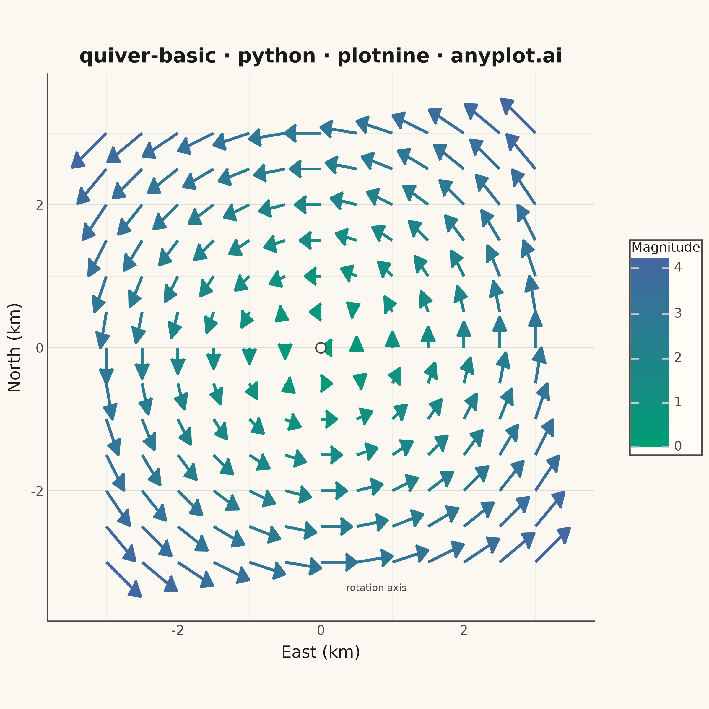
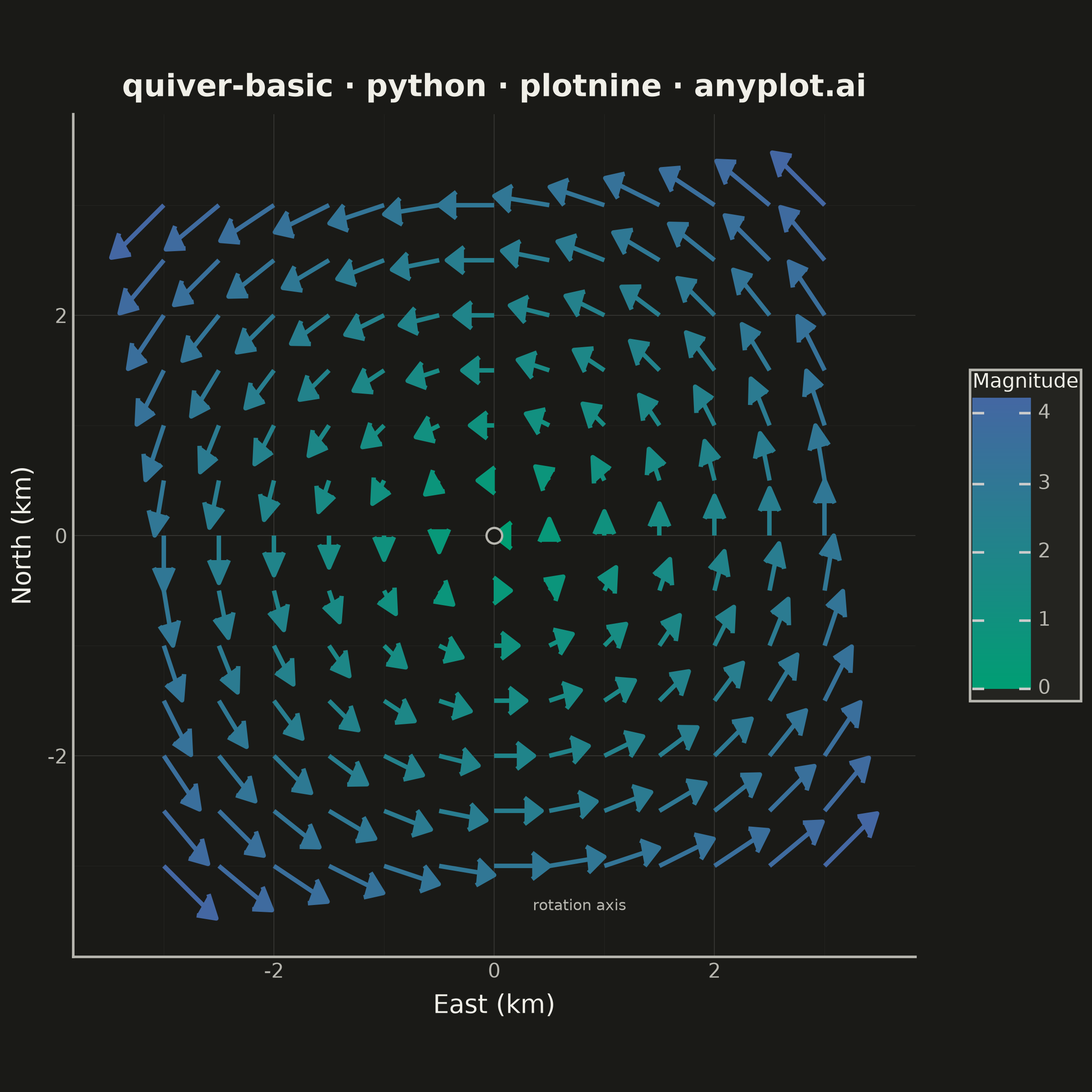
A quiver plot displays vector fields using arrows positioned at grid points. Each arrow represents a vector at that location, with direction indicating the vector's angle and length proportional to its magnitude. This visualization reveals flow patterns, gradients, and field structure in two-dimensional data.
""" anyplot.ai
quiver-basic: Basic Quiver Plot
Library: plotnine 0.15.7 | Python 3.13.14
Quality: 84/100 | Updated: 2026-07-24
"""

import os

import numpy as np
import pandas as pd
from plotnine import (
    aes,
    annotate,
    arrow,
    coord_equal,
    element_blank,
    element_line,
    element_rect,
    element_text,
    geom_segment,
    ggplot,
    labs,
    scale_color_gradient,
    theme,
    theme_minimal,
)


# Theme tokens
THEME = os.getenv("ANYPLOT_THEME", "light")
PAGE_BG = "#FAF8F1" if THEME == "light" else "#1A1A17"
ELEVATED_BG = "#FFFDF6" if THEME == "light" else "#242420"
INK = "#1A1A17" if THEME == "light" else "#F0EFE8"
INK_SOFT = "#4A4A44" if THEME == "light" else "#B8B7B0"

# Data: 13x13 grid rotation flow field (u = -y, v = x) — a slightly coarser
# grid than 15x15 gives corner arrowheads more breathing room.
grid_size = 13
x_vals = np.linspace(-3, 3, grid_size)
y_vals = np.linspace(-3, 3, grid_size)
X, Y = np.meshgrid(x_vals, y_vals)
x = X.flatten()
y = Y.flatten()

# Rotation field: u = -y, v = x (counter-clockwise rotation)
u = -y
v = x

# Magnitude for color encoding
magnitude = np.sqrt(u**2 + v**2)

# Scale arrows for visibility without overlap. A fixed minimum length keeps
# near-origin arrows (magnitude ~ 0) directionally readable instead of
# collapsing to invisible stubs, while length still grows with magnitude.
arrow_scale = 0.14
min_len = 0.08
direction_norm = magnitude + 1e-6
display_len = min_len + arrow_scale * magnitude
u_scaled = u / direction_norm * display_len
v_scaled = v / direction_norm * display_len

# DataFrame with segment start/end and magnitude
df = pd.DataFrame({"x": x, "y": y, "xend": x + u_scaled, "yend": y + v_scaled, "magnitude": magnitude})

# Plot
anyplot_theme = theme(
    figure_size=(6, 6),
    plot_background=element_rect(fill=PAGE_BG, color=PAGE_BG),
    panel_background=element_rect(fill=PAGE_BG),
    panel_grid_major=element_line(color=INK, size=0.3, alpha=0.15),
    panel_grid_minor=element_line(color=INK, size=0.2, alpha=0.05),
    panel_border=element_blank(),
    axis_title=element_text(color=INK, size=10),
    axis_text=element_text(color=INK_SOFT, size=8),
    axis_line=element_line(color=INK_SOFT),
    plot_title=element_text(color=INK, size=12, weight="bold"),
    legend_background=element_rect(fill=ELEVATED_BG, color=INK_SOFT),
    legend_text=element_text(color=INK_SOFT, size=8),
    legend_title=element_text(color=INK, size=8),
    # Dock the colorbar to the plot instead of floating in the right margin.
    legend_box_margin=0,
    legend_margin=2,
    legend_box_spacing=0.05,
    plot_margin=0.01,
)

plot = (
    ggplot(df, aes(x="x", y="y", xend="xend", yend="yend", color="magnitude"))
    + geom_segment(arrow=arrow(length=0.15, type="closed"), size=1.0)
    # Imprint sequential colormap (imprint_seq): brand green -> blue, for
    # single-polarity magnitude data (no meaningful zero-crossing midpoint).
    + scale_color_gradient(low="#009E73", high="#4467A3", name="Magnitude")
    + labs(x="East (km)", y="North (km)", title="quiver-basic · python · plotnine · anyplot.ai")
    + theme_minimal()
    + anyplot_theme
    + coord_equal()
    # Mark the rotation axis at the origin to give the eye a deliberate anchor point.
    + annotate("point", x=0, y=0, color=INK_SOFT, size=3, shape="o", fill=PAGE_BG)
    + annotate("text", x=0.35, y=-3.35, label="rotation axis", color=INK_SOFT, size=6, ha="left")
)

# Save
plot.save(f"plot-{THEME}.png", dpi=400, width=6, height=6, units="in", verbose=False)
Runnable source as JSON, for any HTTP client: https://api.anyplot.ai/specs/quiver-basic/plotnine/code. Any spec id and library id listed in llms-full.txt fit the same URL shape; every URL below is complete and callable.
{
  "spec_id": "quiver-basic",
  "language": "python",
  "library": "plotnine",
  "page": "https://anyplot.ai/quiver-basic/python/plotnine",
  "hub": "https://anyplot.ai/quiver-basic",
  "code_json": "https://api.anyplot.ai/specs/quiver-basic/plotnine/code",
  "spec_json": "https://api.anyplot.ai/specs/quiver-basic",
  "render_light_png": "https://storage.googleapis.com/anyplot-images/plots/quiver-basic/python/plotnine/plot-light.png",
  "render_dark_png": "https://storage.googleapis.com/anyplot-images/plots/quiver-basic/python/plotnine/plot-dark.png",
  "quality_score": 84.0,
  "license": "MIT",
  "guide": "https://anyplot.ai/llms.txt"
}
Part of Basic Quiver Plot on anyplot.ai.