The same plot in 14 other libraries — JavaScript: Chart.js, Apache ECharts, Highcharts, MUI X Charts; Python: Altair, Bokeh, lets-plot, Matplotlib, Plotly, plotnine, Pygal, Seaborn; R: ggplot2; Julia: Makie.jl. Compare all 15 side by side: Basic Raincloud Plot in Python, R, Julia and JavaScript.
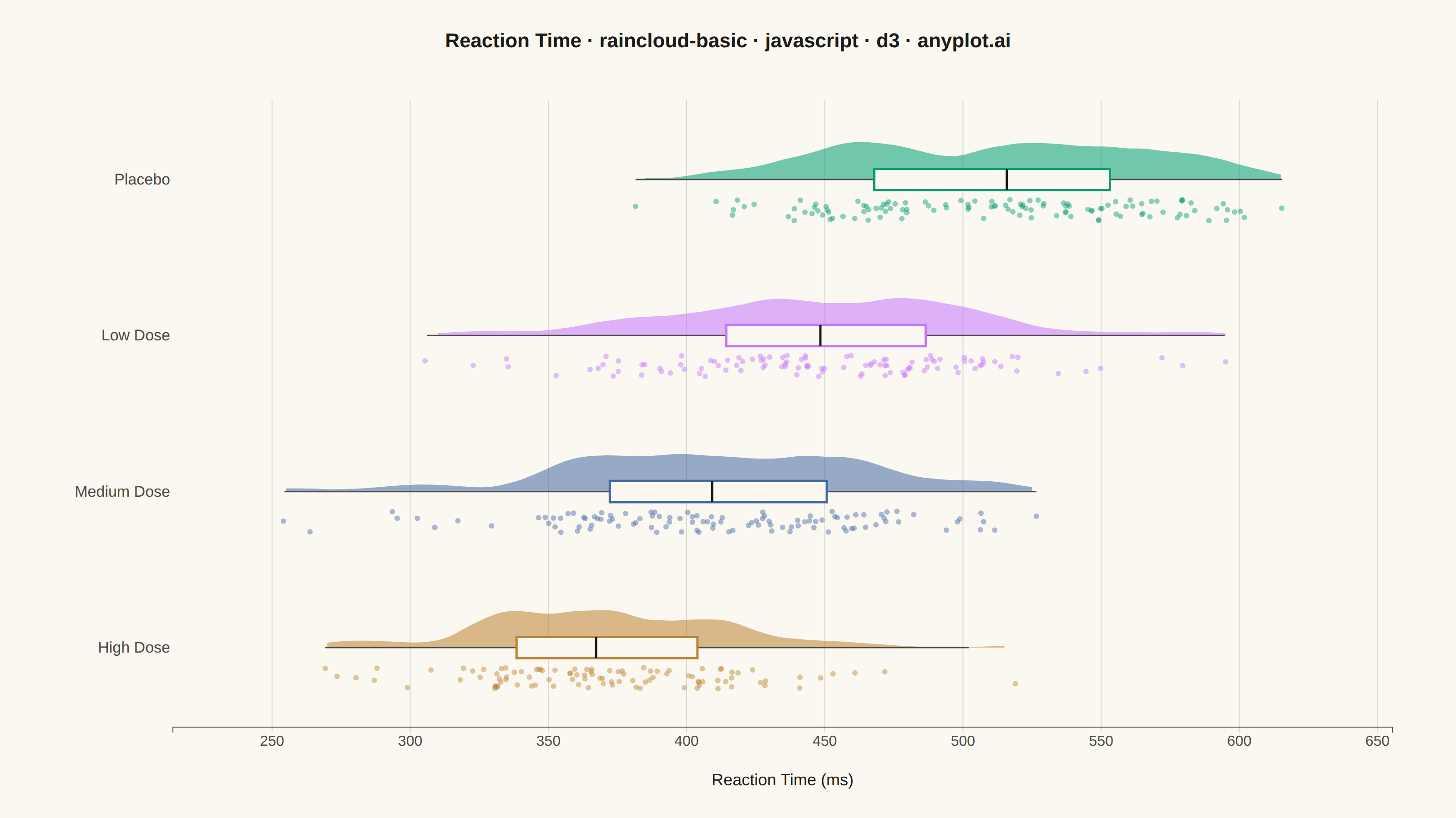
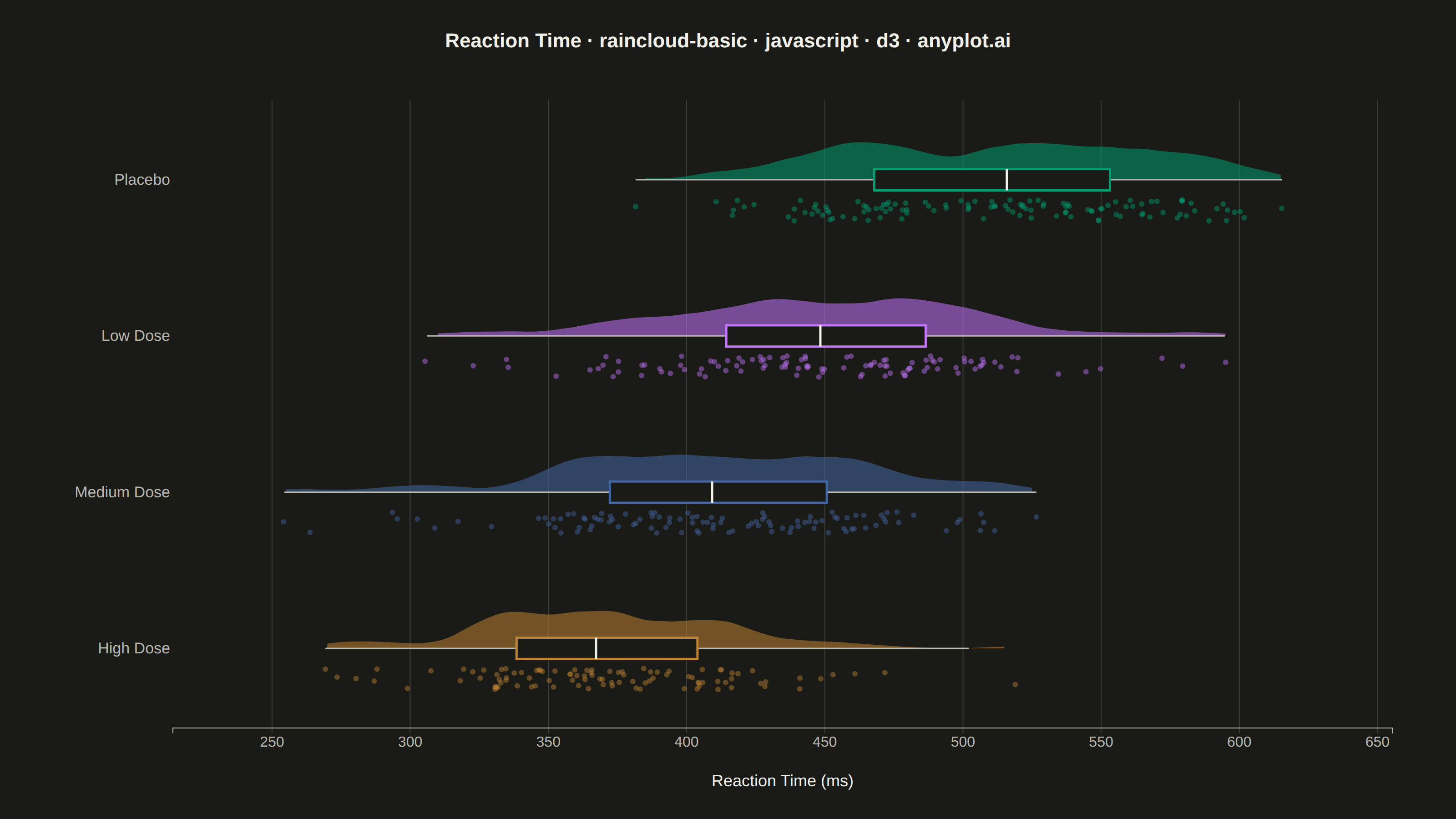
A raincloud plot combines three visualization elements—a half-violin (the "cloud"), jittered strip points (the "rain"), and a box plot—to provide a comprehensive view of data distribution. This hybrid approach shows distribution shape, summary statistics, and individual observations simultaneously, addressing the limitation of box plots that can hide multimodal distributions. Often called the "gold standard" for transparent statistical visualization in scientific publications.
// anyplot.ai
// raincloud-basic: Basic Raincloud Plot
// Library: d3 7.9.0 | JavaScript 22.23.2
// Quality: 91/100 | Created: 2026-08-26

// --- Reproducible RNG (LCG + Box-Muller) ------------------------------------
let seed = 20260826;
const rng = () => {
  seed = (seed * 1664525 + 1013904223) % 4294967296;
  return seed / 4294967296;
};
const randomNormal = (mean, std) => {
  const u1 = Math.max(rng(), 1e-9);
  const u2 = rng();
  const z = Math.sqrt(-2 * Math.log(u1)) * Math.cos(2 * Math.PI * u2);
  return mean + z * std;
};

// --- Data: reaction times (ms) by treatment dose ----------------------------
// Placebo is a mix of two sub-populations (responders / non-responders) to
// show why the cloud reveals multimodality that a box plot alone would hide.
const groups = [
  {
    category: "Placebo",
    values: [
      ...Array.from({ length: 60 }, () => randomNormal(470, 35)),
      ...Array.from({ length: 60 }, () => randomNormal(555, 30)),
    ],
  },
  { category: "Low Dose", values: Array.from({ length: 110 }, () => randomNormal(450, 58)) },
  { category: "Medium Dose", values: Array.from({ length: 110 }, () => randomNormal(410, 52)) },
  { category: "High Dose", values: Array.from({ length: 100 }, () => randomNormal(378, 46)) },
];

const t = window.ANYPLOT_TOKENS;
const { width, height } = window.ANYPLOT_SIZE;
const margin = { top: 110, right: 70, bottom: 100, left: 190 };
const iw = width - margin.left - margin.right;
const ih = height - margin.top - margin.bottom;

const allValues = groups.flatMap((grp) => grp.values);
const x = d3.scaleLinear()
  .domain([d3.min(allValues) - 40, d3.max(allValues) + 40])
  .range([0, iw]);

const y = d3.scaleBand()
  .domain(groups.map((grp) => grp.category))
  .range([0, ih])
  .paddingInner(0.38)
  .paddingOuter(0.2);

const color = d3.scaleOrdinal()
  .domain(groups.map((grp) => grp.category))
  .range(t.palette);

// --- Kernel density estimation for the "cloud" half-violin ------------------
const kernelEpanechnikov = (bandwidth) => (v) =>
  Math.abs((v /= bandwidth)) <= 1 ? (0.75 * (1 - v * v)) / bandwidth : 0;

const kernelDensityEstimator = (kernel, thresholds) => (sample) =>
  thresholds.map((v) => [v, d3.mean(sample, (s) => kernel(v - s))]);

const thresholds = x.ticks(80);

// --- SVG mount ----------------------------------------------------------------
const svg = d3.select("#container").append("svg").attr("width", width).attr("height", height);
const g = svg.append("g").attr("transform", `translate(${margin.left},${margin.top})`);

// --- Vertical gridlines (value axis) -------------------------------------------
g.append("g")
  .selectAll("line")
  .data(x.ticks(8))
  .join("line")
  .attr("x1", (d) => x(d))
  .attr("x2", (d) => x(d))
  .attr("y1", 0)
  .attr("y2", ih)
  .attr("stroke", t.grid)
  .attr("stroke-width", 1);

// --- Draw each category: cloud (above), box (on), rain (below) ----------------
const bandwidth = y.bandwidth();
const halfBand = bandwidth / 2;

for (const grp of groups) {
  const cat = grp.category;
  const values = grp.values.slice().sort(d3.ascending);
  const fill = color(cat);
  const bandTop = y(cat);
  const baseline = bandTop + halfBand;

  // Cloud: KDE curve drawn only above the baseline (half-violin)
  const kdeBandwidth = 1.06 * d3.deviation(values) * Math.pow(values.length, -0.2);
  const kde = kernelDensityEstimator(kernelEpanechnikov(kdeBandwidth), thresholds);
  const density = kde(values).filter(
    (d) => d[0] >= values[0] && d[0] <= values[values.length - 1],
  );
  const maxDensity = d3.max(density, (d) => d[1]) || 1;
  const cloudRise = halfBand * 0.78;
  const densityScale = d3.scaleLinear().domain([0, maxDensity]).range([0, cloudRise]);

  const area = d3.area()
    .x((d) => x(d[0]))
    .y0(baseline)
    .y1((d) => baseline - densityScale(d[1]))
    .curve(d3.curveBasis);

  g.append("path")
    .datum(density)
    .attr("d", area)
    .attr("fill", fill)
    .attr("fill-opacity", 0.55)
    .attr("stroke", "none");

  // Rain: jittered strip points, falling below the baseline
  const boxHalf = Math.min(16, halfBand * 0.22);
  const rainTop = baseline + boxHalf + 10;
  const rainBottom = bandTop + bandwidth - 8;
  const rainSpan = Math.max(12, rainBottom - rainTop);

  g.append("g")
    .selectAll("circle")
    .data(grp.values)
    .join("circle")
    .attr("cx", (d) => x(d))
    .attr("cy", () => rainTop + rng() * rainSpan)
    .attr("r", 3)
    .attr("fill", fill)
    .attr("fill-opacity", 0.45);

  // Box plot: quartiles, whiskers, and median, centered on the baseline
  const q1 = d3.quantileSorted(values, 0.25);
  const median = d3.quantileSorted(values, 0.5);
  const q3 = d3.quantileSorted(values, 0.75);
  const iqr = q3 - q1;
  const loWhisker = Math.max(values[0], q1 - 1.5 * iqr);
  const hiWhisker = Math.min(values[values.length - 1], q3 + 1.5 * iqr);

  g.append("line")
    .attr("x1", x(loWhisker))
    .attr("x2", x(q1))
    .attr("y1", baseline)
    .attr("y2", baseline)
    .attr("stroke", t.inkSoft)
    .attr("stroke-width", 1.5);
  g.append("line")
    .attr("x1", x(q3))
    .attr("x2", x(hiWhisker))
    .attr("y1", baseline)
    .attr("y2", baseline)
    .attr("stroke", t.inkSoft)
    .attr("stroke-width", 1.5);

  g.append("rect")
    .attr("x", x(q1))
    .attr("y", baseline - boxHalf)
    .attr("width", x(q3) - x(q1))
    .attr("height", boxHalf * 2)
    .attr("fill", t.pageBg)
    .attr("stroke", fill)
    .attr("stroke-width", 2.5);

  g.append("line")
    .attr("x1", x(median))
    .attr("x2", x(median))
    .attr("y1", baseline - boxHalf)
    .attr("y2", baseline + boxHalf)
    .attr("stroke", t.ink)
    .attr("stroke-width", 2.5);
}

// --- Axes -----------------------------------------------------------------------
const xAxis = g.append("g").attr("transform", `translate(0,${ih})`).call(d3.axisBottom(x));
const yAxis = g.append("g").call(d3.axisLeft(y).tickSize(0));

for (const ax of [xAxis, yAxis]) {
  ax.selectAll("text").attr("fill", t.inkSoft).style("font-size", "16px");
  ax.selectAll("line").attr("stroke", t.grid);
  ax.select(".domain").attr("stroke", t.inkSoft);
}
yAxis.select(".domain").remove();
yAxis.selectAll("text").style("font-size", "17px");

g.append("text")
  .attr("x", iw / 2)
  .attr("y", ih + 64)
  .attr("text-anchor", "middle")
  .attr("fill", t.ink)
  .style("font-size", "18px")
  .text("Reaction Time (ms)");

// --- Title ------------------------------------------------------------------
svg.append("text")
  .attr("x", width / 2)
  .attr("y", 52)
  .attr("text-anchor", "middle")
  .attr("fill", t.ink)
  .style("font-size", "22px")
  .style("font-weight", "600")
  .text("Reaction Time · raincloud-basic · javascript · d3 · anyplot.ai");
Runnable source as JSON, for any HTTP client: https://api.anyplot.ai/specs/raincloud-basic/d3/code. Any spec id and library id listed in llms-full.txt fit the same URL shape; every URL below is complete and callable.
{
  "spec_id": "raincloud-basic",
  "language": "javascript",
  "library": "d3",
  "page": "https://anyplot.ai/raincloud-basic/javascript/d3",
  "hub": "https://anyplot.ai/raincloud-basic",
  "code_json": "https://api.anyplot.ai/specs/raincloud-basic/d3/code",
  "spec_json": "https://api.anyplot.ai/specs/raincloud-basic",
  "render_light_png": "https://storage.googleapis.com/anyplot-images/plots/raincloud-basic/javascript/d3/plot-light.png",
  "render_dark_png": "https://storage.googleapis.com/anyplot-images/plots/raincloud-basic/javascript/d3/plot-dark.png",
  "interactive_light_html": "https://storage.googleapis.com/anyplot-images/plots/raincloud-basic/javascript/d3/plot-light.html",
  "interactive_dark_html": "https://storage.googleapis.com/anyplot-images/plots/raincloud-basic/javascript/d3/plot-dark.html",
  "quality_score": 91.0,
  "license": "MIT",
  "guide": "https://anyplot.ai/llms.txt"
}
Part of Basic Raincloud Plot on anyplot.ai.