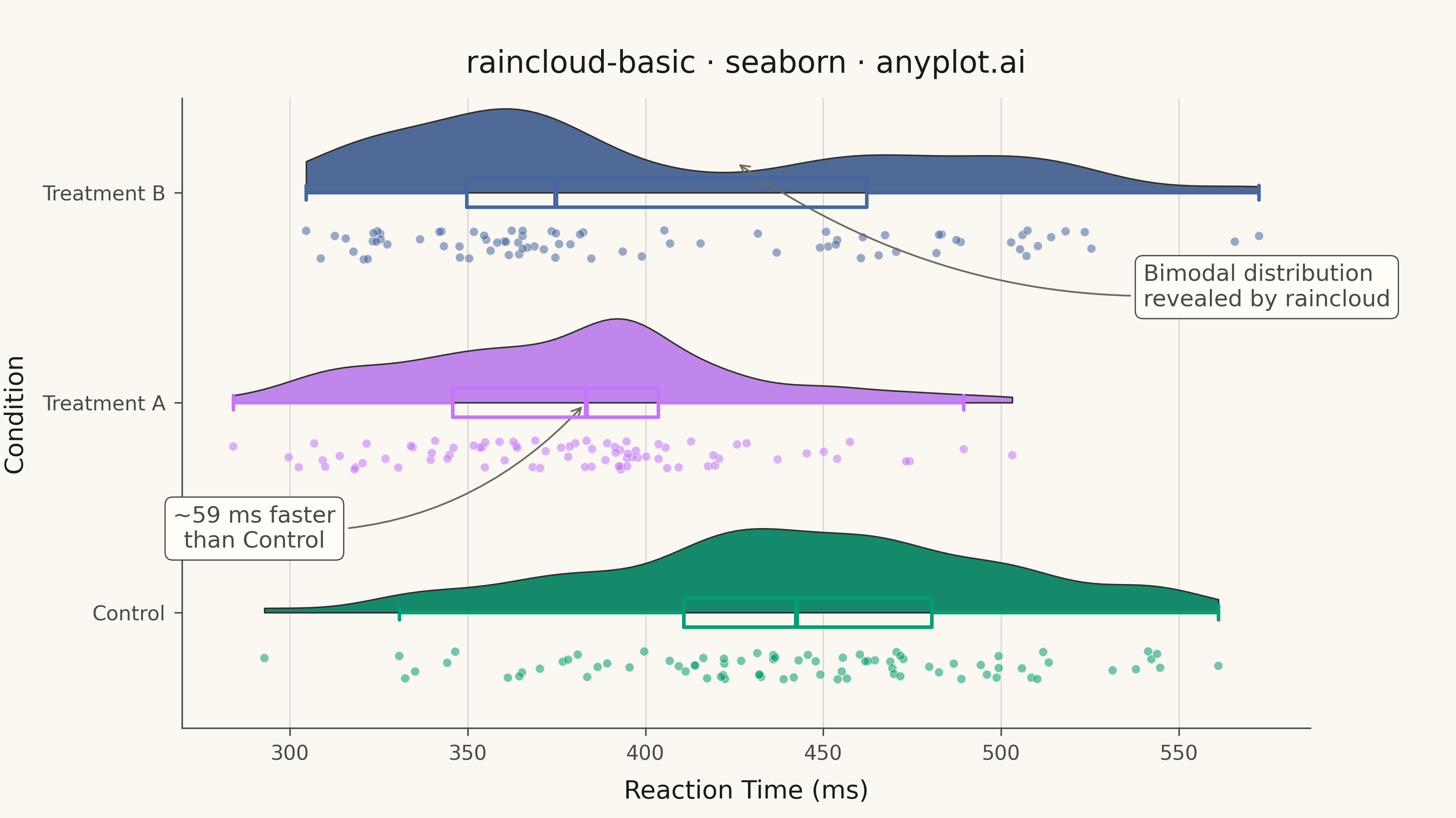
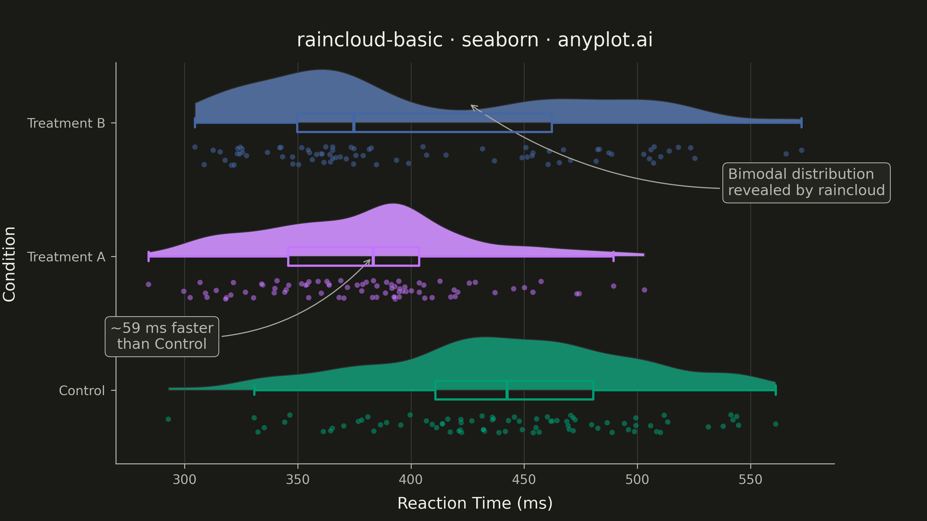
A raincloud plot combines three visualization elements—a half-violin (the "cloud"), jittered strip points (the "rain"), and a box plot—to provide a comprehensive view of data distribution. This hybrid approach shows distribution shape, summary statistics, and individual observations simultaneously, addressing the limitation of box plots that can hide multimodal distributions. Often called the "gold standard" for transparent statistical visualization in scientific publications.
""" anyplot.ai
raincloud-basic: Basic Raincloud Plot
Library: seaborn 0.13.2 | Python 3.13.13
Quality: 93/100 | Updated: 2026-05-26
"""

import os

import matplotlib.pyplot as plt
import numpy as np
import pandas as pd
import seaborn as sns


THEME = os.getenv("ANYPLOT_THEME", "light")
PAGE_BG = "#FAF8F1" if THEME == "light" else "#1A1A17"
ELEVATED_BG = "#FFFDF6" if THEME == "light" else "#242420"
INK = "#1A1A17" if THEME == "light" else "#F0EFE8"
INK_SOFT = "#4A4A44" if THEME == "light" else "#B8B7B0"
INK_MUTED = "#6B6A63" if THEME == "light" else "#A8A79F"

IMPRINT_PALETTE = ["#009E73", "#C475FD", "#4467A3", "#BD8233", "#AE3030", "#2ABCCD", "#954477", "#99B314"]

sns.set_theme(
    style="ticks",
    rc={
        "figure.facecolor": PAGE_BG,
        "axes.facecolor": PAGE_BG,
        "axes.edgecolor": INK_SOFT,
        "axes.labelcolor": INK,
        "text.color": INK,
        "xtick.color": INK_SOFT,
        "ytick.color": INK_SOFT,
        "grid.color": INK,
        "grid.alpha": 0.15,
        "legend.facecolor": ELEVATED_BG,
        "legend.edgecolor": INK_SOFT,
    },
)

# Reaction times (ms) across experimental conditions; Treatment B is bimodal to
# showcase what a raincloud reveals that a box plot would hide.
np.random.seed(42)
control = np.random.normal(450, 60, 80)
treatment_a = np.random.normal(380, 50, 80)
treatment_b = np.concatenate([np.random.normal(350, 30, 50), np.random.normal(480, 40, 30)])

data = pd.DataFrame(
    {
        "Condition": ["Control"] * len(control)
        + ["Treatment A"] * len(treatment_a)
        + ["Treatment B"] * len(treatment_b),
        "Reaction Time": np.concatenate([control, treatment_a, treatment_b]),
    }
)

order = ["Control", "Treatment A", "Treatment B"]
palette = {c: IMPRINT_PALETTE[i] for i, c in enumerate(order)}

fig, ax = plt.subplots(figsize=(8, 4.5), dpi=400)

# Cloud — half-violin, clipped to the upper half above each category baseline
sns.violinplot(
    data=data,
    x="Reaction Time",
    y="Condition",
    hue="Condition",
    palette=palette,
    order=order,
    hue_order=order,
    cut=0,
    inner=None,
    density_norm="width",
    width=0.8,
    linewidth=0.6,
    bw_adjust=0.6,
    ax=ax,
    legend=False,
)
for i, collection in enumerate(ax.collections):
    for path in collection.get_paths():
        v = path.vertices
        v[v[:, 1] < i, 1] = i

n_violin_collections = len(ax.collections)

# Rain — jittered strip points, shifted below the baseline
sns.stripplot(
    data=data,
    x="Reaction Time",
    y="Condition",
    hue="Condition",
    palette=palette,
    order=order,
    hue_order=order,
    jitter=0.07,
    size=3.5,
    alpha=0.55,
    edgecolor=PAGE_BG,
    linewidth=0.3,
    ax=ax,
    legend=False,
)
for collection in ax.collections[n_violin_collections:]:
    offsets = collection.get_offsets()
    offsets[:, 1] -= 0.25
    collection.set_offsets(offsets)
    collection.set_zorder(2)

# Box plot — outlined boxes on the baseline; palette colours the outline,
# whiskers, caps, and median in one stroke (no fragile post-hoc recolouring).
sns.boxplot(
    data=data,
    x="Reaction Time",
    y="Condition",
    hue="Condition",
    palette=palette,
    order=order,
    hue_order=order,
    fill=False,
    width=0.14,
    showfliers=False,
    linewidth=1.4,
    medianprops={"linewidth": 2.0, "solid_capstyle": "butt"},
    ax=ax,
    legend=False,
    zorder=4,
)

ax.set_xlabel("Reaction Time (ms)", fontsize=10, labelpad=6, color=INK)
ax.set_ylabel("Condition", fontsize=10, labelpad=6, color=INK)
ax.set_title("raincloud-basic · seaborn · anyplot.ai", fontsize=12, fontweight="medium", pad=10, color=INK)
ax.tick_params(axis="both", labelsize=8, colors=INK_SOFT, length=3, width=0.6)
ax.grid(True, axis="x", alpha=0.15, linewidth=0.5, color=INK)
ax.set_axisbelow(True)
ax.spines["top"].set_visible(False)
ax.spines["right"].set_visible(False)
ax.spines["left"].set_linewidth(0.6)
ax.spines["bottom"].set_linewidth(0.6)
ax.spines["left"].set_color(INK_SOFT)
ax.spines["bottom"].set_color(INK_SOFT)

ax.set_ylim(-0.55, 2.45)

# Data storytelling
ax.annotate(
    "Bimodal distribution\nrevealed by raincloud",
    xy=(425, 2.15),
    xytext=(540, 1.55),
    fontsize=9,
    fontweight="medium",
    color=INK_SOFT,
    ha="left",
    va="center",
    arrowprops={"arrowstyle": "->", "color": INK_MUTED, "linewidth": 0.7, "connectionstyle": "arc3,rad=-0.2"},
    bbox={"boxstyle": "round,pad=0.35", "facecolor": ELEVATED_BG, "edgecolor": INK_SOFT, "linewidth": 0.5},
)

ta_median = float(np.median(data.loc[data["Condition"] == "Treatment A", "Reaction Time"]))
ctrl_median = float(np.median(data.loc[data["Condition"] == "Control", "Reaction Time"]))
diff_ms = ctrl_median - ta_median

ax.annotate(
    f"~{diff_ms:.0f} ms faster\nthan Control",
    xy=(ta_median, 1.0),
    xytext=(290, 0.4),
    fontsize=9,
    fontweight="medium",
    color=INK_SOFT,
    ha="center",
    va="center",
    arrowprops={"arrowstyle": "->", "color": INK_MUTED, "linewidth": 0.7, "connectionstyle": "arc3,rad=0.25"},
    bbox={"boxstyle": "round,pad=0.35", "facecolor": ELEVATED_BG, "edgecolor": INK_SOFT, "linewidth": 0.5},
)

plt.savefig(f"plot-{THEME}.png", dpi=400, facecolor=PAGE_BG)
Runnable source as JSON, for any HTTP client: https://api.anyplot.ai/specs/raincloud-basic/seaborn/code. Any spec id and library id listed in llms-full.txt fit the same URL shape; every URL below is complete and callable.
{
  "spec_id": "raincloud-basic",
  "language": "python",
  "library": "seaborn",
  "page": "https://anyplot.ai/raincloud-basic/python/seaborn",
  "hub": "https://anyplot.ai/raincloud-basic",
  "code_json": "https://api.anyplot.ai/specs/raincloud-basic/seaborn/code",
  "spec_json": "https://api.anyplot.ai/specs/raincloud-basic",
  "render_light_png": "https://storage.googleapis.com/anyplot-images/plots/raincloud-basic/python/seaborn/plot-light.png",
  "render_dark_png": "https://storage.googleapis.com/anyplot-images/plots/raincloud-basic/python/seaborn/plot-dark.png",
  "quality_score": 93.0,
  "license": "MIT",
  "guide": "https://anyplot.ai/llms.txt"
}
Part of Basic Raincloud Plot on anyplot.ai.