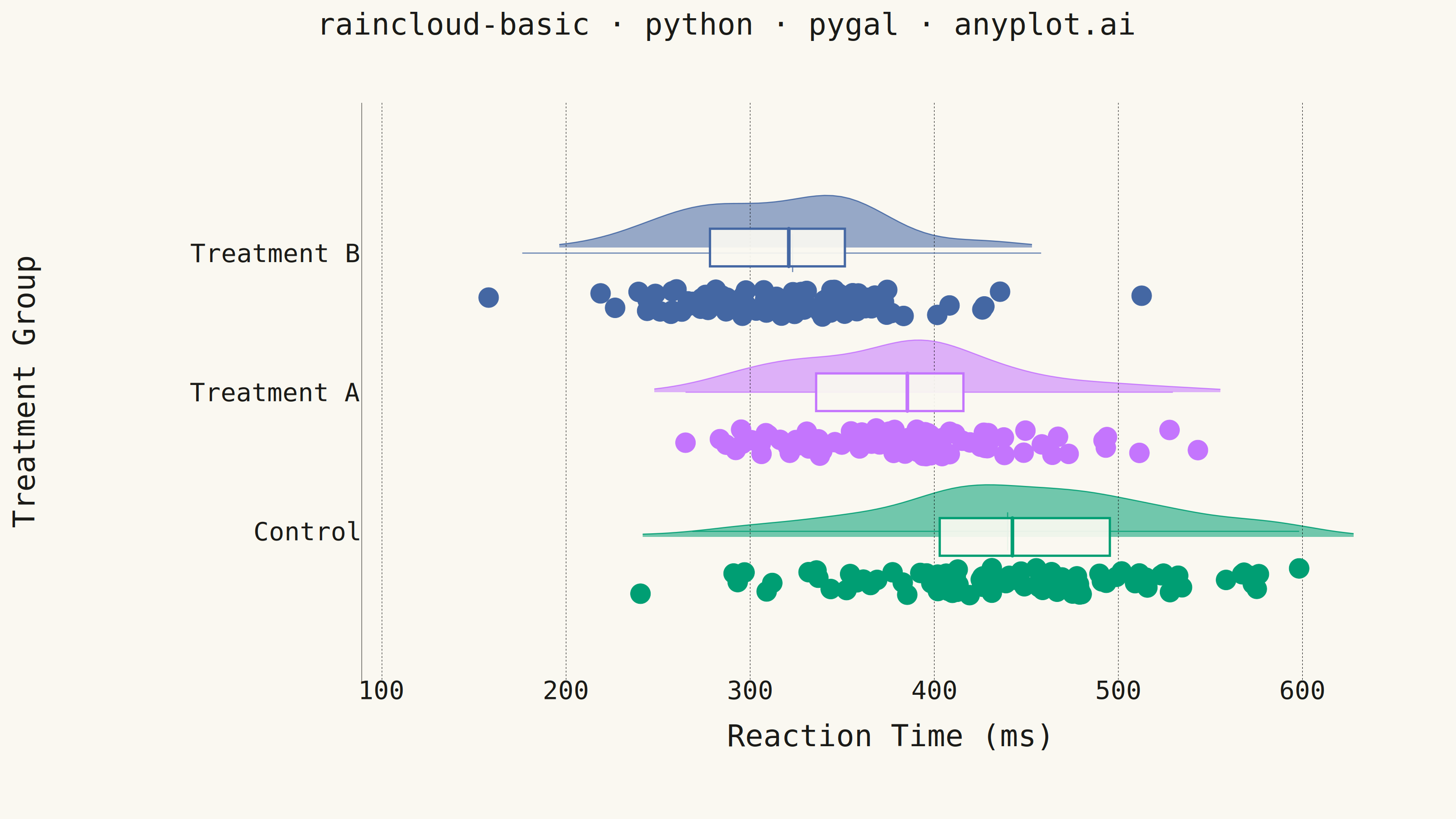
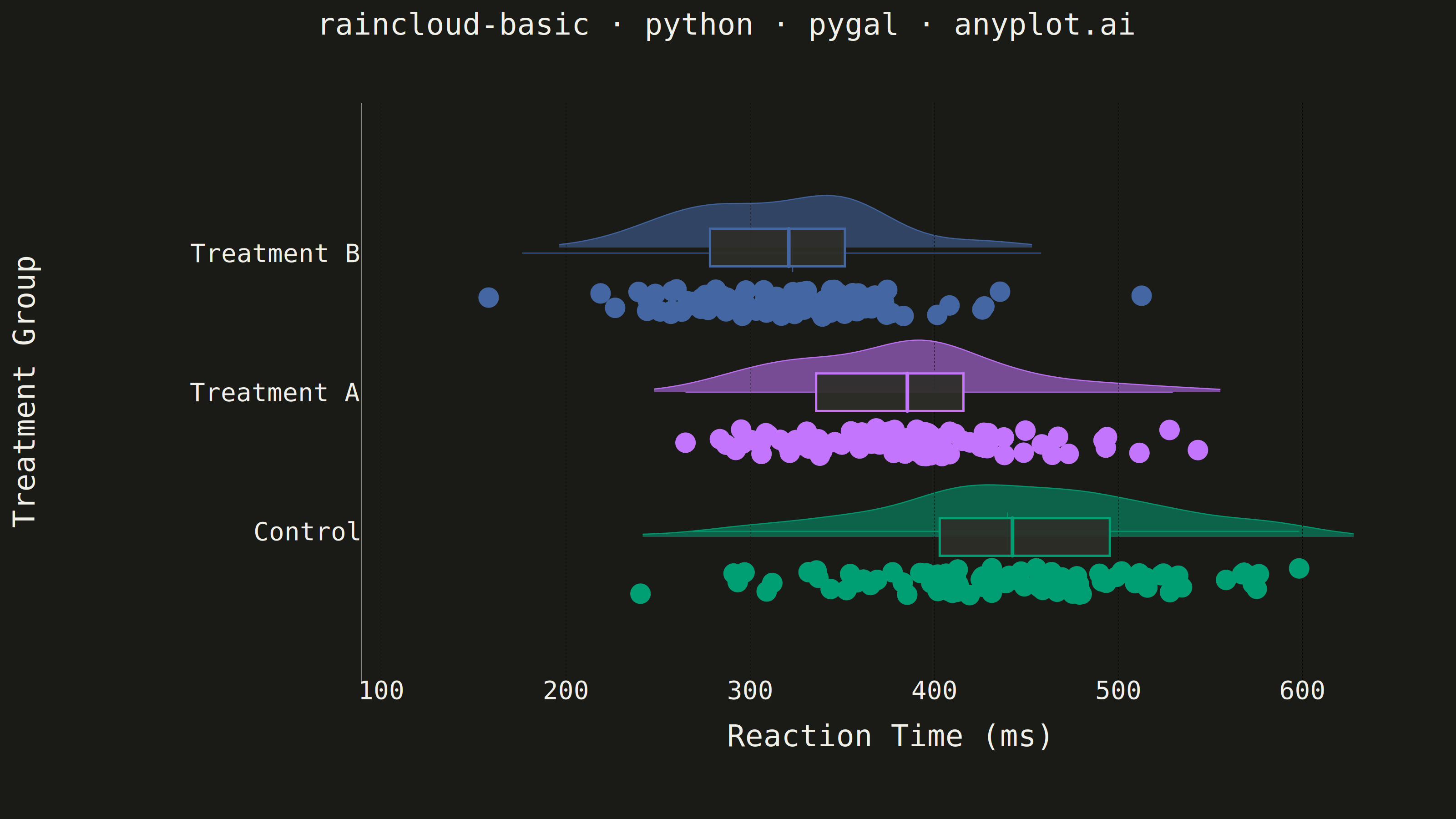
A raincloud plot combines three visualization elements—a half-violin (the "cloud"), jittered strip points (the "rain"), and a box plot—to provide a comprehensive view of data distribution. This hybrid approach shows distribution shape, summary statistics, and individual observations simultaneously, addressing the limitation of box plots that can hide multimodal distributions. Often called the "gold standard" for transparent statistical visualization in scientific publications.
""" anyplot.ai
raincloud-basic: Basic Raincloud Plot
Library: pygal 3.1.0 | Python 3.13.13
Quality: 86/100 | Updated: 2026-05-26
"""

import os
import re

import cairosvg
import numpy as np
import pygal
from pygal.style import Style


# Theme tokens
THEME = os.getenv("ANYPLOT_THEME", "light")
PAGE_BG = "#FAF8F1" if THEME == "light" else "#1A1A17"
INK = "#1A1A17" if THEME == "light" else "#F0EFE8"
INK_SOFT = "#4A4A44" if THEME == "light" else "#B8B7B0"
INK_MUTED = "#6B6A63" if THEME == "light" else "#A8A79F"

# Box-interior fill: in light mode the off-white reads as a hollow box; in dark
# mode PAGE_BG blends into the canvas, so blend toward INK to keep the box
# distinct from the surrounding plot background.
BOX_FILL = "#FAF8F1" if THEME == "light" else "#2E2E29"

IMPRINT_PALETTE = ("#009E73", "#C475FD", "#4467A3", "#BD8233", "#AE3030", "#2ABCCD", "#954477", "#99B314")

# Data — reaction times (ms) for three treatment groups
np.random.seed(42)
data = {
    "Control": np.random.normal(450, 80, 90),
    "Treatment A": np.random.normal(380, 60, 90),
    "Treatment B": np.random.normal(320, 50, 90),
}
group_colors = IMPRINT_PALETTE[: len(data)]

# X-axis bounds with small padding
all_vals = np.concatenate(list(data.values()))
x_lo = float(np.floor((all_vals.min() - 25) / 50) * 50)
x_hi = float(np.ceil((all_vals.max() + 25) / 50) * 50)

# pygal renders one color per series; build the per-series color list so each
# layer (rain, box outline, median line) matches the group color.
series_colors = []
for gc in group_colors:
    series_colors.extend([gc, gc, gc])

custom_style = Style(
    background=PAGE_BG,
    plot_background=PAGE_BG,
    foreground=INK,
    foreground_strong=INK,
    foreground_subtle=INK_MUTED,
    colors=tuple(series_colors),
    title_font_size=66,
    label_font_size=56,
    major_label_font_size=44,
    legend_font_size=44,
    value_font_size=36,
    stroke_width=2.5,
)

CANVAS_W, CANVAS_H = 3200, 1800
MARGIN_LEFT = 340
MARGIN_RIGHT = 90
MARGIN_TOP = 150
MARGIN_BOTTOM = 160

chart = pygal.XY(
    width=CANVAS_W,
    height=CANVAS_H,
    style=custom_style,
    title="raincloud-basic · python · pygal · anyplot.ai",
    x_title="Reaction Time (ms)",
    y_title="Treatment Group",
    show_legend=False,
    stroke=True,
    fill=False,
    dots_size=0,
    show_x_guides=True,
    show_y_guides=False,
    xrange=(x_lo, x_hi),
    range=(0.0, 4.0),
    margin=40,
    margin_left=MARGIN_LEFT,
    margin_right=MARGIN_RIGHT,
    margin_top=MARGIN_TOP,
    margin_bottom=MARGIN_BOTTOM,
    explicit_size=True,
)

# Raincloud layout
cloud_height = 0.36
rain_offset = -0.36
rain_spread = 0.10
n_kde_points = 96
box_hw = 0.13

cloud_polygons = []
box_specs = []
medians = {}

for i, (category, values) in enumerate(data.items()):
    center_y = i + 1
    values = np.array(values)

    # Silverman bandwidth for half-violin KDE
    n = len(values)
    std = float(np.std(values))
    iqr_val = float(np.percentile(values, 75) - np.percentile(values, 25))
    bandwidth = 0.9 * min(std, iqr_val / 1.34) * n ** (-0.2)

    pad = (values.max() - values.min()) * 0.08
    x_kde = np.linspace(values.min() - pad, values.max() + pad, n_kde_points)
    density = np.zeros_like(x_kde)
    for v in values:
        density += np.exp(-0.5 * ((x_kde - v) / bandwidth) ** 2)
    density /= n * bandwidth * np.sqrt(2 * np.pi)

    # Trim KDE tails at 5% of peak for cleaner cloud edges
    peak = density.max()
    keep = np.where(density > peak * 0.05)[0]
    x_kde = x_kde[keep[0] : keep[-1] + 1]
    density = density[keep[0] : keep[-1] + 1]
    density_scaled = density / density.max() * cloud_height

    # Cloud polygon: baseline → top curve → baseline
    poly = [(float(x_kde[0]), float(center_y))]
    poly += [(float(x), float(center_y + d)) for x, d in zip(x_kde, density_scaled, strict=True)]
    poly.append((float(x_kde[-1]), float(center_y)))
    cloud_polygons.append((group_colors[i], poly))

    # Rain: jittered points below baseline
    rng = np.random.default_rng(42 + i)
    jitter = rng.uniform(-rain_spread, rain_spread, len(values))
    rain_points = [
        {"value": (float(v), center_y + rain_offset + float(j)), "label": f"{category}: {v:.0f} ms"}
        for j, v in zip(jitter, values, strict=True)
    ]
    chart.add(f"{category} rain", rain_points, stroke=False, fill=False, dots_size=22)

    # Box plot statistics
    median = float(np.median(values))
    q1 = float(np.percentile(values, 25))
    q3 = float(np.percentile(values, 75))
    iqr = q3 - q1
    w_lo = float(max(values.min(), q1 - 1.5 * iqr))
    w_hi = float(min(values.max(), q3 + 1.5 * iqr))
    medians[category] = median
    box_specs.append((group_colors[i], center_y, q1, q3, median, w_lo, w_hi))

    # Whisker line (added via pygal so the box has a native-rendered backbone)
    chart.add(
        "", [(w_lo, center_y), (w_hi, center_y)], stroke=True, fill=False, show_dots=False, stroke_style={"width": 4}
    )
    # Median rule (drawn as a vertical line inside the box via two XY points)
    chart.add(
        "",
        [(median, center_y - box_hw * 1.05), (median, center_y + box_hw * 1.05)],
        stroke=True,
        fill=False,
        show_dots=False,
        stroke_style={"width": 10},
    )

chart.y_labels = [
    {"value": 0.0, "label": ""},
    {"value": 1.0, "label": "Control"},
    {"value": 2.0, "label": "Treatment A"},
    {"value": 3.0, "label": "Treatment B"},
    {"value": 4.0, "label": ""},
]

# Render base SVG
base_svg = chart.render().decode("utf-8")

# Extract the actual plot-area transform + dimensions from the rendered SVG
# (pygal computes them from title/axis-label space, so reading them back beats
# trying to predict them).
plot_g = re.search(r'<g\s+transform="translate\(([0-9.]+)[,\s]+([0-9.]+)\)"\s+class="plot">', base_svg)
plot_tx, plot_ty = float(plot_g.group(1)), float(plot_g.group(2))

plot_rect = re.search(
    r'class="plot">.*?<rect[^>]*width="([0-9.]+)"[^>]*height="([0-9.]+)"'
    r'[^>]*class="background"',
    base_svg,
    re.DOTALL,
)
plot_w, plot_h = float(plot_rect.group(1)), float(plot_rect.group(2))

# Data → plot-local SVG pixel mapping (SVG y is inverted relative to data y)
x_scale = plot_w / (x_hi - x_lo)
x_offset = -x_lo * x_scale
y_data_lo, y_data_hi = 0.0, 4.0
y_scale = -plot_h / (y_data_hi - y_data_lo)
y_offset = -y_data_hi * y_scale


def to_svg(px, py):
    return px * x_scale + x_offset, py * y_scale + y_offset


# Cloud polygons — injected inside the plot group (uses plot-local coords).
# Fill is the full polygon (closed back to baseline); the stroke is drawn
# separately as a polyline along only the curved top edge so the baseline
# closure doesn't show as a visible horizontal line.
clouds_svg = '<g class="raincloud-clouds">'
for color, poly in cloud_polygons:
    pts = " ".join(f"{x:.1f},{y:.1f}" for x, y in (to_svg(px, py) for px, py in poly))
    # Curve-only stroke: skip the first and last vertices (the baseline endpoints).
    curve_pts = " ".join(f"{x:.1f},{y:.1f}" for x, y in (to_svg(px, py) for px, py in poly[1:-1]))
    clouds_svg += (
        f'<polygon points="{pts}" fill="{color}" fill-opacity="0.55" stroke="none"/>'
        f'<polyline points="{curve_pts}" fill="none" '
        f'stroke="{color}" stroke-width="2.5" stroke-opacity="0.9"/>'
    )
clouds_svg += "</g>"

bg_marker = 'class="background"'
first_bg = base_svg.find(bg_marker)
second_bg = base_svg.find(bg_marker, first_bg + 1)
bg_end = base_svg.find("/>", second_bg) + 2
base_svg = base_svg[:bg_end] + clouds_svg + base_svg[bg_end:]

# Box-plot rectangles — drawn in absolute SVG coords (outside plot group)
boxes_svg = '<g class="raincloud-boxes">'
for color, cy, q1, q3, median, _w_lo, _w_hi in box_specs:
    bx1, by1 = to_svg(q1, cy + box_hw)
    bx2, by2 = to_svg(q3, cy - box_hw)
    bx, by = bx1 + plot_tx, by1 + plot_ty
    bw, bh = bx2 - bx1, by2 - by1
    mx, _ = to_svg(median, cy)
    mx += plot_tx
    box_top_y = by
    box_bot_y = by + bh
    boxes_svg += (
        f'<rect x="{bx:.1f}" y="{by:.1f}" width="{bw:.1f}" height="{bh:.1f}" '
        f'fill="{BOX_FILL}" fill-opacity="0.92" '
        f'stroke="{color}" stroke-width="5"/>'
        f'<line x1="{mx:.1f}" y1="{box_top_y:.1f}" '
        f'x2="{mx:.1f}" y2="{box_bot_y:.1f}" '
        f'stroke="{color}" stroke-width="8" stroke-linecap="round"/>'
    )
boxes_svg += "</g>"

svg_out = base_svg.replace("</svg>", f"{boxes_svg}\n</svg>")

# Save outputs
with open(f"plot-{THEME}.svg", "w") as f:
    f.write(svg_out)

cairosvg.svg2png(
    bytestring=svg_out.encode("utf-8"), write_to=f"plot-{THEME}.png", output_width=CANVAS_W, output_height=CANVAS_H
)

with open(f"plot-{THEME}.html", "wb") as f:
    f.write(svg_out.encode("utf-8"))
Runnable source as JSON, for any HTTP client: https://api.anyplot.ai/specs/raincloud-basic/pygal/code. Any spec id and library id listed in llms-full.txt fit the same URL shape; every URL below is complete and callable.
{
  "spec_id": "raincloud-basic",
  "language": "python",
  "library": "pygal",
  "page": "https://anyplot.ai/raincloud-basic/python/pygal",
  "hub": "https://anyplot.ai/raincloud-basic",
  "code_json": "https://api.anyplot.ai/specs/raincloud-basic/pygal/code",
  "spec_json": "https://api.anyplot.ai/specs/raincloud-basic",
  "render_light_png": "https://storage.googleapis.com/anyplot-images/plots/raincloud-basic/python/pygal/plot-light.png",
  "render_dark_png": "https://storage.googleapis.com/anyplot-images/plots/raincloud-basic/python/pygal/plot-dark.png",
  "interactive_light_html": "https://storage.googleapis.com/anyplot-images/plots/raincloud-basic/python/pygal/plot-light.html",
  "interactive_dark_html": "https://storage.googleapis.com/anyplot-images/plots/raincloud-basic/python/pygal/plot-dark.html",
  "quality_score": 86.0,
  "license": "MIT",
  "guide": "https://anyplot.ai/llms.txt"
}
Part of Basic Raincloud Plot on anyplot.ai.