The same plot in 14 other libraries — Python: Altair, Bokeh, lets-plot, Matplotlib, Plotly, plotnine, Pygal, Seaborn; R: ggplot2; JavaScript: Chart.js, D3.js, Apache ECharts, Highcharts, MUI X Charts. Compare all 15 side by side: Basic Ridgeline Plot in Python, R, Julia and JavaScript.
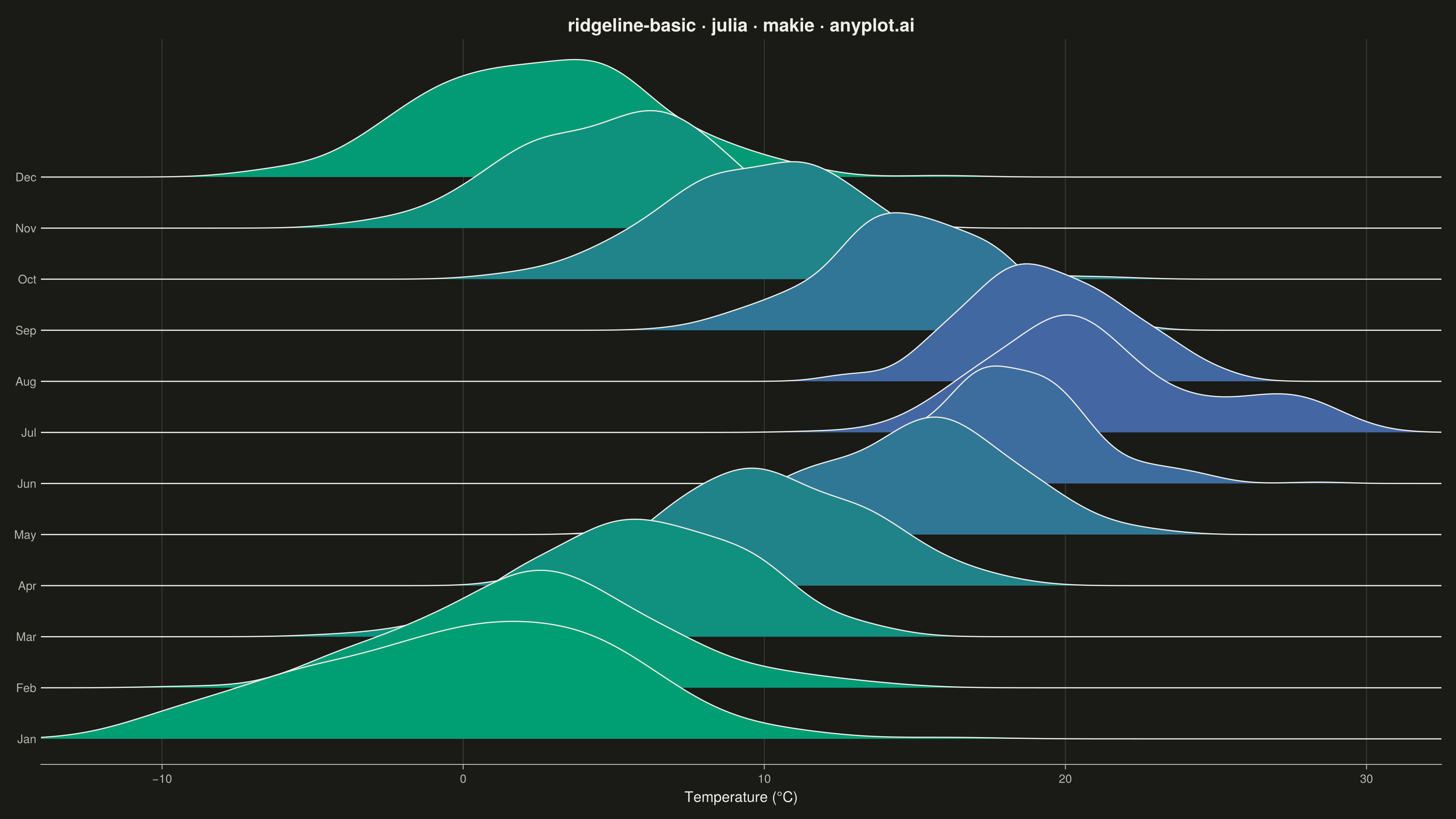
A ridgeline plot (also known as Joy Plot, named after the Joy Division album cover) displays the distribution of multiple groups by stacking partially overlapping density curves vertically. This creates a mountain ridge appearance that allows efficient comparison of many distributions simultaneously while maintaining a compact and visually striking presentation.
# anyplot.ai
# ridgeline-basic: Basic Ridgeline Plot
# Library: makie 0.21.9 | Julia 1.11.9
# Quality: 95/100 | Created: 2026-07-25

using CairoMakie
using Colors
using Random
using Statistics

Random.seed!(42)

# --- Theme tokens ------------------------------------------------------------
THEME    = get(ENV, "ANYPLOT_THEME", "light")
PAGE_BG  = THEME == "light" ? colorant"#FAF8F1" : colorant"#1A1A17"
INK      = THEME == "light" ? colorant"#1A1A17" : colorant"#F0EFE8"
INK_SOFT = THEME == "light" ? colorant"#4A4A44" : colorant"#B8B7B0"

# Imprint sequential colormap (brand green -> blue) — the 12 ridges form a
# seasonal cycle, so a gradient reads better here than 12 discrete hues.
IMPRINT_SEQ = cgrad([colorant"#009E73", colorant"#4467A3"])

# --- Data ----------------------------------------------------------------------
# Daily mean temperature normals for a temperate climate (approx. Berlin, DE)
months = ["Jan", "Feb", "Mar", "Apr", "May", "Jun",
          "Jul", "Aug", "Sep", "Oct", "Nov", "Dec"]
mean_temp = [1.6, 2.5, 6.1, 10.4, 14.6, 17.9, 19.8, 19.4, 14.9, 10.2, 5.5, 2.5]
std_temp = [4.0, 4.0, 3.7, 3.3, 3.0, 2.7, 2.5, 2.5, 2.8, 3.2, 3.6, 3.9]
n_obs = 250

# Most months are a single symmetric Gaussian; Jan and Jul get an extra
# minority component (a cold-snap / heat-spike bump) so the ridgeline also
# demonstrates shape differences, not just shift/spread differences.
n_bump = 40
daily_temps = Vector{Vector{Float64}}(undef, 12)
for m in 1:12
    main = randn(n_obs - (m in (1, 7) ? n_bump : 0)) .* std_temp[m] .+ mean_temp[m]
    if m == 1
        cold_snap = randn(n_bump) .* (std_temp[m] * 0.5) .+ (mean_temp[m] - 9.0)
        daily_temps[m] = vcat(main, cold_snap)
    elseif m == 7
        heat_spike = randn(n_bump) .* (std_temp[m] * 0.5) .+ (mean_temp[m] + 7.5)
        daily_temps[m] = vcat(main, heat_spike)
    else
        daily_temps[m] = main
    end
end

# Shared temperature grid for the kernel density estimate
grid_min = minimum(minimum.(daily_temps)) - 3.0
grid_max = maximum(maximum.(daily_temps)) + 3.0
temp_grid = range(grid_min, grid_max; length = 300)

# Gaussian KDE per month (Silverman bandwidth), each normalized to a shared
# ridge height so the vertical overlap stays consistent across all 12 ridges
ridge_step = 1.0
ridge_height = 2.3
baselines = [(m - 1) * ridge_step for m in 1:12]
ridge_curves = Vector{Vector{Float64}}(undef, 12)
for m in 1:12
    data = daily_temps[m]
    bandwidth = 1.06 * std(data) * length(data)^(-1 / 5)
    density = [sum(exp.(-0.5 .* ((t .- data) ./ bandwidth) .^ 2)) for t in temp_grid]
    density ./= (length(data) * bandwidth * sqrt(2π))
    ridge_curves[m] = density ./ maximum(density) .* ridge_height .+ baselines[m]
end

# --- Plot ------------------------------------------------------------------
fig = Figure(size = (1600, 900), fontsize = 14, backgroundcolor = PAGE_BG)

ax = Axis(
    fig[1, 1];
    title = "ridgeline-basic · julia · makie · anyplot.ai",
    titlesize = 20,
    titlecolor = INK,
    xlabel = "Temperature (°C)",
    xlabelsize = 16,
    xlabelcolor = INK,
    xticklabelsize = 13,
    xticklabelcolor = INK_SOFT,
    xtickcolor = INK_SOFT,
    yticks = (baselines, months),
    yticklabelsize = 13,
    yticklabelcolor = INK_SOFT,
    yticksvisible = false,
    backgroundcolor = PAGE_BG,
    topspinevisible = false,
    rightspinevisible = false,
    leftspinevisible = false,
    bottomspinecolor = INK_SOFT,
    xgridcolor = RGBAf(INK.r, INK.g, INK.b, 0.15),
    ygridvisible = false,
)

# Color keyed to actual mean temperature (min-max normalized), not month
# index, so the gradient reinforces the warm/cold story instead of just
# re-encoding the chronological order the Y-axis already shows.
temp_norm = (mean_temp .- minimum(mean_temp)) ./ (maximum(mean_temp) - minimum(mean_temp))

for m in 12:-1:1
    ridge_color = get(IMPRINT_SEQ, temp_norm[m])
    band!(ax, temp_grid, fill(baselines[m], length(temp_grid)), ridge_curves[m];
          color = ridge_color)
    lines!(ax, temp_grid, ridge_curves[m]; color = INK, linewidth = 1.3)
end

ylims!(ax, -0.5, baselines[end] + ridge_height + 0.4)
xlims!(ax, grid_min, grid_max)

# --- Save --------------------------------------------------------------------
save("plot-$(THEME).png", fig; px_per_unit = 2)
Runnable source as JSON, for any HTTP client: https://api.anyplot.ai/specs/ridgeline-basic/makie/code. Any spec id and library id listed in llms-full.txt fit the same URL shape; every URL below is complete and callable.
{
  "spec_id": "ridgeline-basic",
  "language": "julia",
  "library": "makie",
  "page": "https://anyplot.ai/ridgeline-basic/julia/makie",
  "hub": "https://anyplot.ai/ridgeline-basic",
  "code_json": "https://api.anyplot.ai/specs/ridgeline-basic/makie/code",
  "spec_json": "https://api.anyplot.ai/specs/ridgeline-basic",
  "render_light_png": "https://storage.googleapis.com/anyplot-images/plots/ridgeline-basic/julia/makie/plot-light.png",
  "render_dark_png": "https://storage.googleapis.com/anyplot-images/plots/ridgeline-basic/julia/makie/plot-dark.png",
  "quality_score": 95.0,
  "license": "MIT",
  "guide": "https://anyplot.ai/llms.txt"
}
Part of Basic Ridgeline Plot on anyplot.ai.