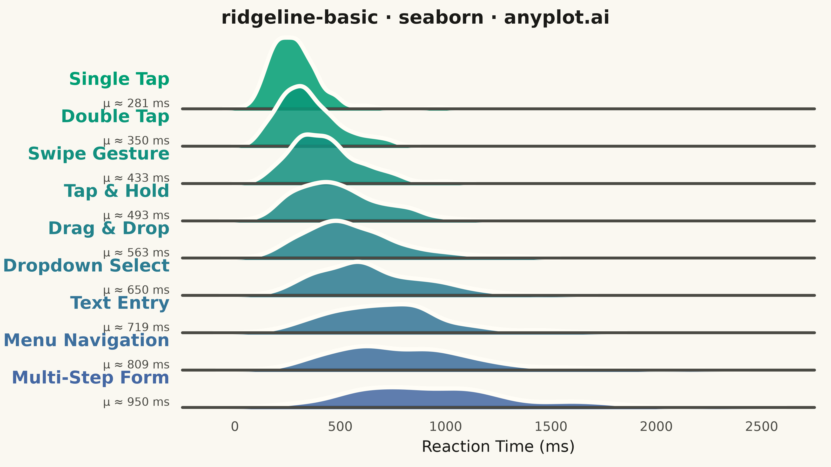
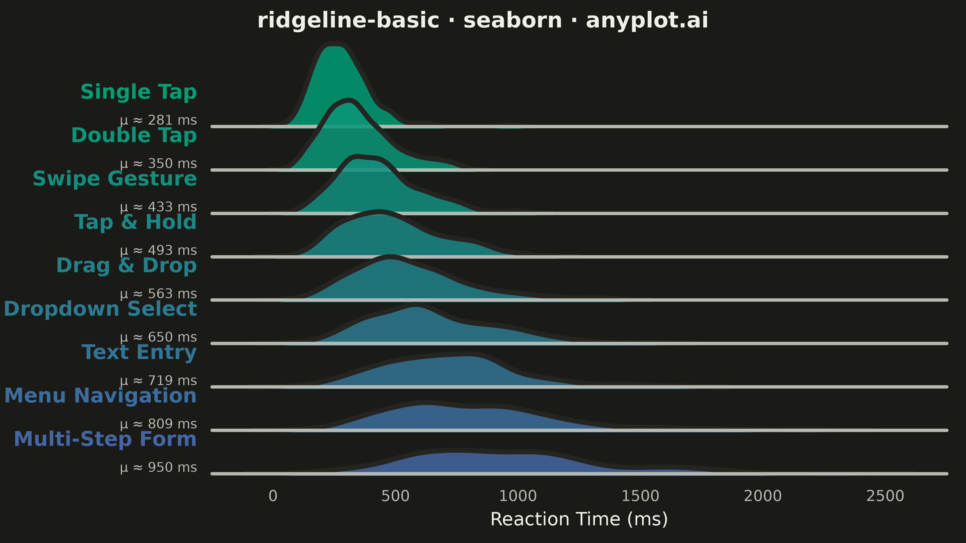
A ridgeline plot (also known as Joy Plot, named after the Joy Division album cover) displays the distribution of multiple groups by stacking partially overlapping density curves vertically. This creates a mountain ridge appearance that allows efficient comparison of many distributions simultaneously while maintaining a compact and visually striking presentation.
""" anyplot.ai
ridgeline-basic: Basic Ridgeline Plot
Library: seaborn 0.13.2 | Python 3.13.14
Quality: 93/100 | Updated: 2026-07-25
"""

import os

import matplotlib.pyplot as plt
import numpy as np
import pandas as pd
import seaborn as sns
from matplotlib.colors import LinearSegmentedColormap


# Theme tokens
THEME = os.getenv("ANYPLOT_THEME", "light")
PAGE_BG = "#FAF8F1" if THEME == "light" else "#1A1A17"
ELEVATED_BG = "#FFFDF6" if THEME == "light" else "#242420"
INK = "#1A1A17" if THEME == "light" else "#F0EFE8"
INK_SOFT = "#4A4A44" if THEME == "light" else "#B8B7B0"

# Data - UI task reaction times, ordered by rising interaction complexity
np.random.seed(42)

tasks = [
    "Single Tap",
    "Double Tap",
    "Swipe Gesture",
    "Tap & Hold",
    "Drag & Drop",
    "Dropdown Select",
    "Text Entry",
    "Menu Navigation",
    "Multi-Step Form",
]

mean_ms = [280, 350, 420, 480, 560, 630, 720, 810, 950]
gamma_shape = 6  # moderate right skew, characteristic of human reaction-time distributions

data = []
for task, mu in zip(tasks, mean_ms, strict=True):
    reaction_times = np.random.gamma(shape=gamma_shape, scale=mu / gamma_shape, size=180)
    for value in reaction_times:
        data.append({"task": task, "reaction_time": value})

df = pd.DataFrame(data)

# Imprint sequential colormap (brand green -> blue): single-polarity gradient tracks rising task complexity
imprint_seq = LinearSegmentedColormap.from_list("imprint_seq", ["#009E73", "#4467A3"])
palette = [imprint_seq(t) for t in np.linspace(0, 1, len(tasks))]

# Configure seaborn: transparent axes so figure background shows through
sns.set_theme(
    style="white",
    rc={
        "axes.facecolor": (0, 0, 0, 0),
        "figure.facecolor": PAGE_BG,
        "text.color": INK,
        "axes.labelcolor": INK,
        "xtick.color": INK_SOFT,
        "ytick.color": INK_SOFT,
    },
)

# FacetGrid ridgeline layout (simplest task at top -> most complex task at bottom)
g = sns.FacetGrid(df, row="task", hue="task", aspect=15, height=0.6, palette=palette, row_order=tasks, hue_order=tasks)

# Filled density curves
g.map(sns.kdeplot, "reaction_time", bw_adjust=0.8, clip_on=False, fill=True, alpha=0.85, linewidth=2.5)

# Outline in ELEVATED_BG creates visible separation between overlapping ridges on both themes
g.map(sns.kdeplot, "reaction_time", bw_adjust=0.8, clip_on=False, color=ELEVATED_BG, linewidth=3)

# Baseline
g.map(plt.axhline, y=0, linewidth=2, linestyle="-", color=INK_SOFT, clip_on=False)


def label(x, color, label):
    ax = plt.gca()
    ax.text(
        -0.02, 0.38, label, fontsize=12, fontweight="bold", color=color, ha="right", va="center", transform=ax.transAxes
    )
    ax.text(
        -0.02,
        0.06,
        f"μ ≈ {x.mean():.0f} ms",
        fontsize=10,
        color=INK_SOFT,
        ha="right",
        va="center",
        transform=ax.transAxes,
    )


g.map(label, "reaction_time")

# Overlap and cleanup
g.figure.subplots_adjust(hspace=-0.5)
g.set_titles("")
g.set(yticks=[], ylabel="")
g.despine(bottom=True, left=True)

g.axes[-1, 0].set_xlabel("Reaction Time (ms)", fontsize=11, color=INK)
g.axes[-1, 0].tick_params(axis="x", labelsize=9, colors=INK_SOFT)

g.figure.set_size_inches(8, 4.5)
g.figure.patch.set_facecolor(PAGE_BG)
g.figure.suptitle("ridgeline-basic · python · seaborn · anyplot.ai", fontsize=13, y=0.98, fontweight="bold", color=INK)

plt.savefig(f"plot-{THEME}.png", dpi=400, facecolor=PAGE_BG)
Runnable source as JSON, for any HTTP client: https://api.anyplot.ai/specs/ridgeline-basic/seaborn/code. Any spec id and library id listed in llms-full.txt fit the same URL shape; every URL below is complete and callable.
{
  "spec_id": "ridgeline-basic",
  "language": "python",
  "library": "seaborn",
  "page": "https://anyplot.ai/ridgeline-basic/python/seaborn",
  "hub": "https://anyplot.ai/ridgeline-basic",
  "code_json": "https://api.anyplot.ai/specs/ridgeline-basic/seaborn/code",
  "spec_json": "https://api.anyplot.ai/specs/ridgeline-basic",
  "render_light_png": "https://storage.googleapis.com/anyplot-images/plots/ridgeline-basic/python/seaborn/plot-light.png",
  "render_dark_png": "https://storage.googleapis.com/anyplot-images/plots/ridgeline-basic/python/seaborn/plot-dark.png",
  "quality_score": 93.0,
  "license": "MIT",
  "guide": "https://anyplot.ai/llms.txt"
}
Part of Basic Ridgeline Plot on anyplot.ai.