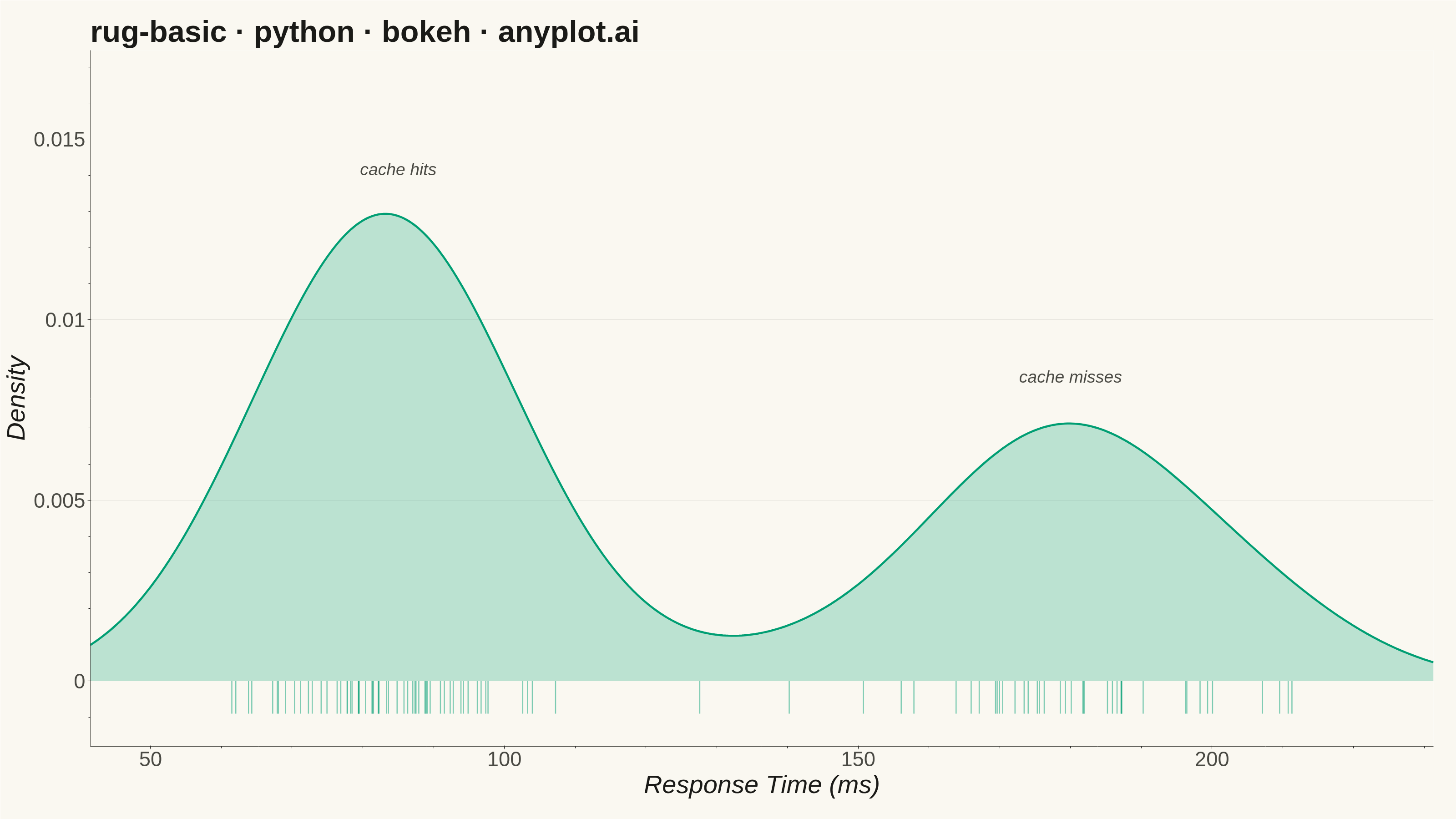
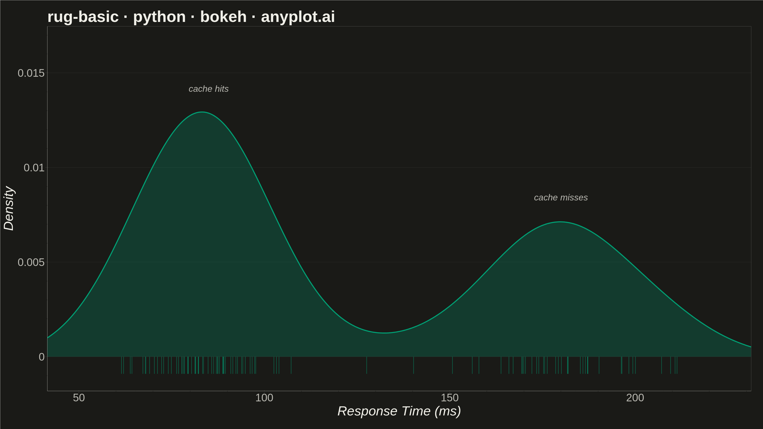
A rug plot displays individual data points as small tick marks along an axis, typically at the bottom or side of another plot. Unlike histograms or density plots that bin data, rug plots show the exact location of every observation. They reveal clustering patterns, gaps in data, and the precise distribution of values with minimal visual footprint.
""" anyplot.ai
rug-basic: Basic Rug Plot
Library: bokeh 3.9.1 | Python 3.13.14
Quality: 89/100 | Updated: 2026-07-25
"""

import io
import os
import sys
import time
from pathlib import Path


# Prevent this file's directory from shadowing the installed bokeh package
sys.path = [p for p in sys.path if os.path.abspath(p or os.getcwd()) != os.path.dirname(os.path.abspath(__file__))]

import numpy as np
from bokeh.io import output_file, save
from bokeh.models import ColumnDataSource, HoverTool, Label, Range1d
from bokeh.plotting import figure
from PIL import Image
from scipy import stats
from selenium import webdriver
from selenium.webdriver.chrome.options import Options


# Theme tokens
THEME = os.getenv("ANYPLOT_THEME", "light")
PAGE_BG = "#FAF8F1" if THEME == "light" else "#1A1A17"
INK = "#1A1A17" if THEME == "light" else "#F0EFE8"
INK_SOFT = "#4A4A44" if THEME == "light" else "#B8B7B0"
BRAND = "#009E73"  # Imprint palette position 1 — always first series

# Data — bimodal API response times (ms) showing clustering patterns
np.random.seed(42)
cluster1 = np.random.normal(85, 12, 60)  # Fast responses (cache hits)
cluster2 = np.random.normal(180, 20, 40)  # Slower responses (cache misses)
values = np.concatenate([cluster1, cluster2])

# KDE curve
kde = stats.gaussian_kde(values, bw_method=0.3)
x_smooth = np.linspace(values.min() - 20, values.max() + 20, 500)
kde_y = kde(x_smooth)

# Rug ticks sit just below y=0
rug_top = 0.0
rug_bottom = -kde_y.max() * 0.07
rug_mid = (rug_top + rug_bottom) / 2

# Sources
kde_source = ColumnDataSource(data={"x": x_smooth, "y": kde_y})
rug_source = ColumnDataSource(
    data={"x": values, "y0": np.full(len(values), rug_bottom), "y1": np.full(len(values), rug_top)}
)
rug_hover_source = ColumnDataSource(data={"x": values, "y_mid": np.full(len(values), rug_mid)})

# Figure — 3200×1800 landscape
p = figure(
    width=3200,
    height=1800,
    title="rug-basic · python · bokeh · anyplot.ai",
    x_axis_label="Response Time (ms)",
    y_axis_label="Density",
    toolbar_location=None,
    min_border_bottom=160,
    min_border_left=180,
    min_border_top=110,
    min_border_right=50,
)

# KDE density — filled area plus edge line
p.varea(x="x", y1=0, y2="y", source=kde_source, fill_color=BRAND, fill_alpha=0.25)
p.line("x", "y", source=kde_source, line_color=BRAND, line_width=4.5)

# Rug ticks along the x-axis — thin line_width keeps individual ticks
# distinguishable even where the fast-response cluster packs densely
p.segment(x0="x", y0="y0", x1="x", y1="y1", source=rug_source, line_color=BRAND, line_width=2.5, line_alpha=0.5)

# Invisible scatter over the rug ticks — hit target for hover, showcasing
# Bokeh's interactive strength (exact response time per observation)
rug_hits = p.scatter(x="x", y="y_mid", source=rug_hover_source, size=24, fill_alpha=0, line_alpha=0)
hover = HoverTool(renderers=[rug_hits], tooltips=[("Response Time", "@x{0.0} ms")], mode="vline")
p.add_tools(hover)

# Axis ranges
p.x_range = Range1d(values.min() - 20, values.max() + 20)
p.y_range = Range1d(rug_bottom * 2.0, kde_y.max() * 1.35)

# Cluster call-outs — guide the viewer through the bimodal story
for mode_x, mode_label in ((85, "cache hits"), (180, "cache misses")):
    mode_y = float(kde(mode_x)[0])
    p.add_layout(
        Label(
            x=mode_x,
            y=mode_y + kde_y.max() * 0.08,
            text=mode_label,
            text_align="center",
            text_font_size="28pt",
            text_font_style="italic",
            text_color=INK_SOFT,
        )
    )

# Text sizing — canonical bokeh values for 3200×1800
p.title.text_font_size = "50pt"
p.xaxis.axis_label_text_font_size = "42pt"
p.yaxis.axis_label_text_font_size = "42pt"
p.xaxis.major_label_text_font_size = "34pt"
p.yaxis.major_label_text_font_size = "34pt"

# Theme-adaptive chrome
p.background_fill_color = PAGE_BG
p.border_fill_color = PAGE_BG
p.outline_line_color = None  # drop the frame for a cleaner, less "default" look

p.title.text_color = INK
p.xaxis.axis_label_text_color = INK
p.yaxis.axis_label_text_color = INK
p.xaxis.major_label_text_color = INK_SOFT
p.yaxis.major_label_text_color = INK_SOFT
p.xaxis.axis_line_color = INK_SOFT
p.yaxis.axis_line_color = INK_SOFT
p.xaxis.major_tick_line_color = INK_SOFT
p.yaxis.major_tick_line_color = INK_SOFT

p.xgrid.grid_line_color = None
p.ygrid.grid_line_color = INK
p.ygrid.grid_line_alpha = 0.10

# Save HTML (interactive catalog artifact)
output_file(f"plot-{THEME}.html")
save(p)

# Screenshot with headless Chrome (Selenium 4 / Selenium Manager).
# Chrome's internal UI overhead shrinks the viewport below --window-size by ~139 px.
# Use a taller window (H + 200 buffer) so the viewport is >= H, then crop to exact dims.
W, H = 3200, 1800
opts = Options()
for arg in (
    "--headless=new",
    "--no-sandbox",
    "--disable-dev-shm-usage",
    "--disable-gpu",
    f"--window-size={W},{H + 200}",
    "--hide-scrollbars",
    "--force-device-scale-factor=1",
):
    opts.add_argument(arg)
driver = webdriver.Chrome(options=opts)
driver.set_window_size(W, H + 200)
driver.get(f"file://{Path(f'plot-{THEME}.html').resolve()}")
time.sleep(3)
raw = driver.get_screenshot_as_png()
driver.quit()
img = Image.open(io.BytesIO(raw)).crop((0, 0, W, H))
img.save(f"plot-{THEME}.png")
Runnable source as JSON, for any HTTP client: https://api.anyplot.ai/specs/rug-basic/bokeh/code. Any spec id and library id listed in llms-full.txt fit the same URL shape; every URL below is complete and callable.
{
  "spec_id": "rug-basic",
  "language": "python",
  "library": "bokeh",
  "page": "https://anyplot.ai/rug-basic/python/bokeh",
  "hub": "https://anyplot.ai/rug-basic",
  "code_json": "https://api.anyplot.ai/specs/rug-basic/bokeh/code",
  "spec_json": "https://api.anyplot.ai/specs/rug-basic",
  "render_light_png": "https://storage.googleapis.com/anyplot-images/plots/rug-basic/python/bokeh/plot-light.png",
  "render_dark_png": "https://storage.googleapis.com/anyplot-images/plots/rug-basic/python/bokeh/plot-dark.png",
  "interactive_light_html": "https://storage.googleapis.com/anyplot-images/plots/rug-basic/python/bokeh/plot-light.html",
  "interactive_dark_html": "https://storage.googleapis.com/anyplot-images/plots/rug-basic/python/bokeh/plot-dark.html",
  "quality_score": 89.0,
  "license": "MIT",
  "guide": "https://anyplot.ai/llms.txt"
}
Part of Basic Rug Plot on anyplot.ai.