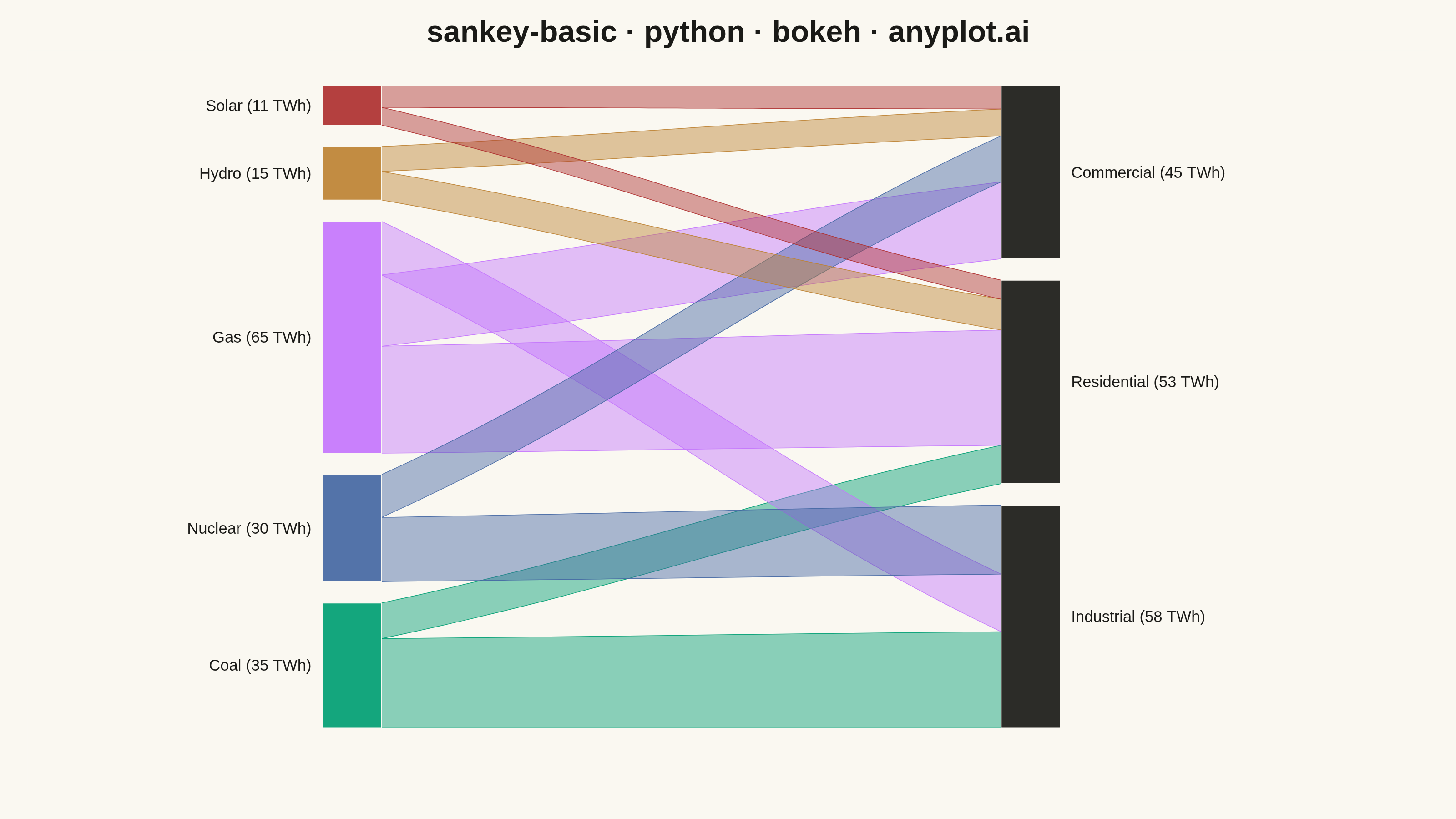
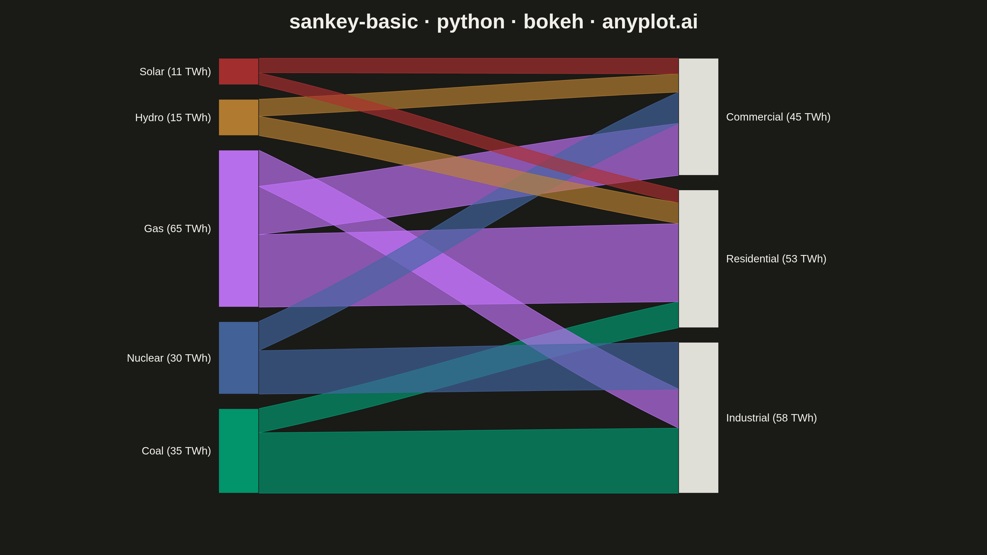
A Sankey diagram visualizes flow or transfer between nodes using links with widths proportional to flow values. It excels at showing how quantities distribute from sources to destinations, revealing patterns in resource allocation, process flows, and system transitions. The diagram makes it easy to identify major pathways and compare relative magnitudes of different flows.
""" anyplot.ai
sankey-basic: Basic Sankey Diagram
Library: bokeh 3.9.1 | Python 3.13.14
Quality: 89/100 | Updated: 2026-07-25
"""

import os
import sys
import time
from pathlib import Path


_script_dir = os.path.dirname(os.path.abspath(__file__))
sys.path = [p for p in sys.path if os.path.abspath(p or ".") != _script_dir]

import numpy as np
from bokeh.io import output_file, save
from bokeh.models import ColumnDataSource, HoverTool, Label
from bokeh.plotting import figure
from selenium import webdriver
from selenium.webdriver.chrome.options import Options


# Theme tokens
THEME = os.getenv("ANYPLOT_THEME", "light")
PAGE_BG = "#FAF8F1" if THEME == "light" else "#1A1A17"
INK = "#1A1A17" if THEME == "light" else "#F0EFE8"
INK_SOFT = "#4A4A44" if THEME == "light" else "#B8B7B0"
FLOW_ALPHA = 0.45 if THEME == "light" else 0.65  # dark bg needs more opacity to keep ribbons visible

# Imprint palette — first source always #009E73
IMPRINT_PALETTE = ["#009E73", "#C475FD", "#4467A3", "#BD8233", "#AE3030"]
NEUTRAL = INK  # theme-adaptive anchor for sector (target) nodes — structural, not categorical

# Data - Energy flow from sources to sectors (TWh)
flows = [
    {"source": "Coal", "target": "Industrial", "value": 25},
    {"source": "Coal", "target": "Residential", "value": 10},
    {"source": "Gas", "target": "Residential", "value": 30},
    {"source": "Gas", "target": "Commercial", "value": 20},
    {"source": "Gas", "target": "Industrial", "value": 15},
    {"source": "Nuclear", "target": "Industrial", "value": 18},
    {"source": "Nuclear", "target": "Commercial", "value": 12},
    {"source": "Hydro", "target": "Residential", "value": 8},
    {"source": "Hydro", "target": "Commercial", "value": 7},
    {"source": "Solar", "target": "Residential", "value": 5},
    {"source": "Solar", "target": "Commercial", "value": 6},
]

# Extract unique sources and targets (preserve order)
sources = []
targets = []
for f in flows:
    if f["source"] not in sources:
        sources.append(f["source"])
    if f["target"] not in targets:
        targets.append(f["target"])

# Source colors: Imprint palette in canonical order (encounter order, independent
# of the crossing-minimized visual stacking order computed below)
source_colors = {s: IMPRINT_PALETTE[i] for i, s in enumerate(sources)}

# Calculate totals for node sizing
source_totals = {s: sum(f["value"] for f in flows if f["source"] == s) for s in sources}
target_totals = {t: sum(f["value"] for f in flows if f["target"] == t) for t in targets}


# Crossing-minimization: reorder the vertical stacking of source/target nodes via
# a barycenter heuristic (each node's position converges toward the weighted-average
# position of the nodes it connects to) so ribbons cross less and the flow reads
# with a clearer focal point.
def _barycenter_reorder(this_side, other_order, connections):
    other_index = {name: i for i, name in enumerate(other_order)}
    scores = {}
    for name in this_side:
        conns = connections[name]
        total = sum(v for _, v in conns)
        scores[name] = sum(other_index[o] * v for o, v in conns) / total if total else other_index.get(name, 0)
    return sorted(this_side, key=lambda n: scores[n])


source_to_targets = {s: [(f["target"], f["value"]) for f in flows if f["source"] == s] for s in sources}
target_to_sources = {t: [(f["source"], f["value"]) for f in flows if f["target"] == t] for t in targets}

ordered_sources = list(sources)
ordered_targets = list(targets)
for _ in range(4):
    ordered_targets = _barycenter_reorder(ordered_targets, ordered_sources, target_to_sources)
    ordered_sources = _barycenter_reorder(ordered_sources, ordered_targets, source_to_targets)

# Layout parameters (data-space percent units, independent of canvas pixels)
left_x = 0
right_x = 100
node_width = 8
node_gap = 3
total_height = 100
padding_y = 5

# Calculate node positions for sources (left side)
source_height_total = sum(source_totals.values())
scale_src = (total_height - 2 * padding_y - (len(sources) - 1) * node_gap) / source_height_total

source_nodes = {}
current_y = padding_y
for s in ordered_sources:
    height = source_totals[s] * scale_src
    source_nodes[s] = {"x": left_x, "y": current_y, "height": height, "value": source_totals[s]}
    current_y += height + node_gap

# Calculate node positions for targets (right side)
target_height_total = sum(target_totals.values())
scale_tgt = (total_height - 2 * padding_y - (len(targets) - 1) * node_gap) / target_height_total

target_nodes = {}
current_y = padding_y
for t in ordered_targets:
    height = target_totals[t] * scale_tgt
    target_nodes[t] = {"x": right_x - node_width, "y": current_y, "height": height, "value": target_totals[t]}
    current_y += height + node_gap

# Track flow offsets for stacking flows at each node
source_offsets = dict.fromkeys(sources, 0.0)
target_offsets = dict.fromkeys(targets, 0.0)

# Build flow ribbons as bezier patches, collected into a ColumnDataSource so
# HoverTool can read per-flow source/target/value on mouseover.
flow_xs, flow_ys, flow_source, flow_target, flow_value, flow_color = [], [], [], [], [], []
for f in flows:
    src = f["source"]
    tgt = f["target"]
    value = f["value"]

    src_node = source_nodes[src]
    tgt_node = target_nodes[tgt]

    src_flow_height = (value / source_totals[src]) * src_node["height"]
    tgt_flow_height = (value / target_totals[tgt]) * tgt_node["height"]

    x0 = src_node["x"] + node_width
    y0_bottom = src_node["y"] + source_offsets[src]
    y0_top = y0_bottom + src_flow_height

    x1 = tgt_node["x"]
    y1_bottom = tgt_node["y"] + target_offsets[tgt]
    y1_top = y1_bottom + tgt_flow_height

    source_offsets[src] += src_flow_height
    target_offsets[tgt] += tgt_flow_height

    t = np.linspace(0, 1, 60)
    cx0 = x0 + (x1 - x0) * 0.4
    cx1 = x0 + (x1 - x0) * 0.6

    x_path = (1 - t) ** 3 * x0 + 3 * (1 - t) ** 2 * t * cx0 + 3 * (1 - t) * t**2 * cx1 + t**3 * x1
    y_bottom = (1 - t) * y0_bottom + t * y1_bottom
    y_top = (1 - t) * y0_top + t * y1_top

    flow_xs.append(list(x_path) + list(x_path[::-1]))
    flow_ys.append(list(y_top) + list(y_bottom[::-1]))
    flow_source.append(src)
    flow_target.append(tgt)
    flow_value.append(value)
    flow_color.append(source_colors[src])

flow_cds = ColumnDataSource(
    data={
        "xs": flow_xs,
        "ys": flow_ys,
        "flow_source": flow_source,
        "flow_target": flow_target,
        "flow_value": flow_value,
        "flow_color": flow_color,
    }
)

# Nodes (sources + sectors) as a single ColumnDataSource for hover + rendering
node_name = list(ordered_sources) + list(ordered_targets)
node_role = ["Source"] * len(ordered_sources) + ["Sector"] * len(ordered_targets)
node_left = [source_nodes[s]["x"] for s in ordered_sources] + [target_nodes[t]["x"] for t in ordered_targets]
node_right = [source_nodes[s]["x"] + node_width for s in ordered_sources] + [
    target_nodes[t]["x"] + node_width for t in ordered_targets
]
node_bottom = [source_nodes[s]["y"] for s in ordered_sources] + [target_nodes[t]["y"] for t in ordered_targets]
node_top = [source_nodes[s]["y"] + source_nodes[s]["height"] for s in ordered_sources] + [
    target_nodes[t]["y"] + target_nodes[t]["height"] for t in ordered_targets
]
node_value = [source_nodes[s]["value"] for s in ordered_sources] + [target_nodes[t]["value"] for t in ordered_targets]
node_color = [source_colors[s] for s in ordered_sources] + [NEUTRAL] * len(ordered_targets)

nodes_cds = ColumnDataSource(
    data={
        "name": node_name,
        "role": node_role,
        "left": node_left,
        "right": node_right,
        "bottom": node_bottom,
        "top": node_top,
        "value": node_value,
        "color": node_color,
    }
)

# Plot — canonical 3200x1800 landscape canvas
p = figure(
    width=3200,
    height=1800,
    title="sankey-basic · python · bokeh · anyplot.ai",
    # Generous L/R x_range margin — Label text clips at the frame/range boundary,
    # not the canvas edge, so overflow room must live in x_range, not min_border_*.
    x_range=(-40, 150),
    y_range=(-4, 100),
    tools="",
    toolbar_location=None,  # bokeh's default toolbar adds ~30-50px above the canvas
    min_border_bottom=60,
    min_border_left=60,
    min_border_top=110,
    min_border_right=60,
)

flow_renderer = p.patches(
    "xs",
    "ys",
    source=flow_cds,
    fill_color="flow_color",
    fill_alpha=FLOW_ALPHA,
    line_color="flow_color",
    # More opaque, slightly thicker stroke than the fill so a ribbon's own edge
    # stays traceable through alpha-blended crossings instead of dissolving into
    # a blended hue.
    line_alpha=0.9,
    line_width=1.5,
)

node_renderer = p.quad(
    left="left",
    right="right",
    bottom="bottom",
    top="top",
    source=nodes_cds,
    fill_color="color",
    fill_alpha=0.92,
    line_color=PAGE_BG,
    line_width=2,
)

p.add_tools(
    HoverTool(
        renderers=[flow_renderer], tooltips=[("Flow", "@flow_source → @flow_target"), ("Volume", "@flow_value TWh")]
    )
)
p.add_tools(HoverTool(renderers=[node_renderer], tooltips=[("Node", "@name (@role)"), ("Total", "@value TWh")]))

# Node labels — source nodes left-aligned outward, target nodes right-aligned outward
for s in ordered_sources:
    node = source_nodes[s]
    label = Label(
        x=node["x"] - 1.5,
        y=node["y"] + node["height"] / 2,
        text=f"{s} ({node['value']} TWh)",
        text_font_size="26pt",
        text_align="right",
        text_baseline="middle",
        text_color=INK,
        text_font="helvetica",
    )
    p.add_layout(label)

for t in ordered_targets:
    node = target_nodes[t]
    label = Label(
        x=node["x"] + node_width + 1.5,
        y=node["y"] + node["height"] / 2,
        text=f"{t} ({node['value']} TWh)",
        text_font_size="26pt",
        text_align="left",
        text_baseline="middle",
        text_color=INK,
        text_font="helvetica",
    )
    p.add_layout(label)

# Style — theme-adaptive chrome
p.title.text_font_size = "50pt"
p.title.text_color = INK
p.title.align = "center"
p.title.text_font = "helvetica"

p.xaxis.visible = False
p.yaxis.visible = False
p.xgrid.visible = False
p.ygrid.visible = False
p.outline_line_color = None

p.background_fill_color = PAGE_BG
p.border_fill_color = PAGE_BG

# Save — write the interactive HTML, then screenshot it with headless Chrome.
# bokeh.io.export_png is avoided here (unreliable chromedriver resolution);
# Selenium + CDP viewport pinning matches the exact 3200x1800 canvas.
output_file(f"plot-{THEME}.html")
save(p)

W, H = 3200, 1800
opts = Options()
for arg in (
    "--headless=new",
    "--no-sandbox",
    "--disable-dev-shm-usage",
    "--disable-gpu",
    f"--window-size={W},{H}",
    "--hide-scrollbars",
):
    opts.add_argument(arg)
driver = webdriver.Chrome(options=opts)
driver.set_window_size(W, H)
driver.get(f"file://{Path(f'plot-{THEME}.html').resolve()}")
driver.execute_cdp_cmd(
    "Emulation.setDeviceMetricsOverride", {"width": W, "height": H, "deviceScaleFactor": 1, "mobile": False}
)
# Zero out the default page margin/background so no stray edge pixel of the
# browser's default white page bleeds through around the themed canvas.
driver.execute_script(
    f"document.documentElement.style.background='{PAGE_BG}';"
    f"document.body.style.background='{PAGE_BG}';"
    "document.body.style.margin='0';"
    "document.body.style.overflow='hidden';"
)
time.sleep(3)  # let bokeh's JS render the canvas
driver.save_screenshot(f"plot-{THEME}.png")
driver.quit()
Runnable source as JSON, for any HTTP client: https://api.anyplot.ai/specs/sankey-basic/bokeh/code. Any spec id and library id listed in llms-full.txt fit the same URL shape; every URL below is complete and callable.
{
  "spec_id": "sankey-basic",
  "language": "python",
  "library": "bokeh",
  "page": "https://anyplot.ai/sankey-basic/python/bokeh",
  "hub": "https://anyplot.ai/sankey-basic",
  "code_json": "https://api.anyplot.ai/specs/sankey-basic/bokeh/code",
  "spec_json": "https://api.anyplot.ai/specs/sankey-basic",
  "render_light_png": "https://storage.googleapis.com/anyplot-images/plots/sankey-basic/python/bokeh/plot-light.png",
  "render_dark_png": "https://storage.googleapis.com/anyplot-images/plots/sankey-basic/python/bokeh/plot-dark.png",
  "interactive_light_html": "https://storage.googleapis.com/anyplot-images/plots/sankey-basic/python/bokeh/plot-light.html",
  "interactive_dark_html": "https://storage.googleapis.com/anyplot-images/plots/sankey-basic/python/bokeh/plot-dark.html",
  "quality_score": 89.0,
  "license": "MIT",
  "guide": "https://anyplot.ai/llms.txt"
}
Part of Basic Sankey Diagram on anyplot.ai.