The same plot in 13 other libraries — Python: Altair, Bokeh, lets-plot, Matplotlib, Plotly, plotnine, Pygal, Seaborn; Julia: Makie.jl; JavaScript: D3.js, Apache ECharts, Highcharts, MUI X Charts. Compare all 14 side by side: Basic Sankey Diagram in Python, R, Julia and JavaScript.
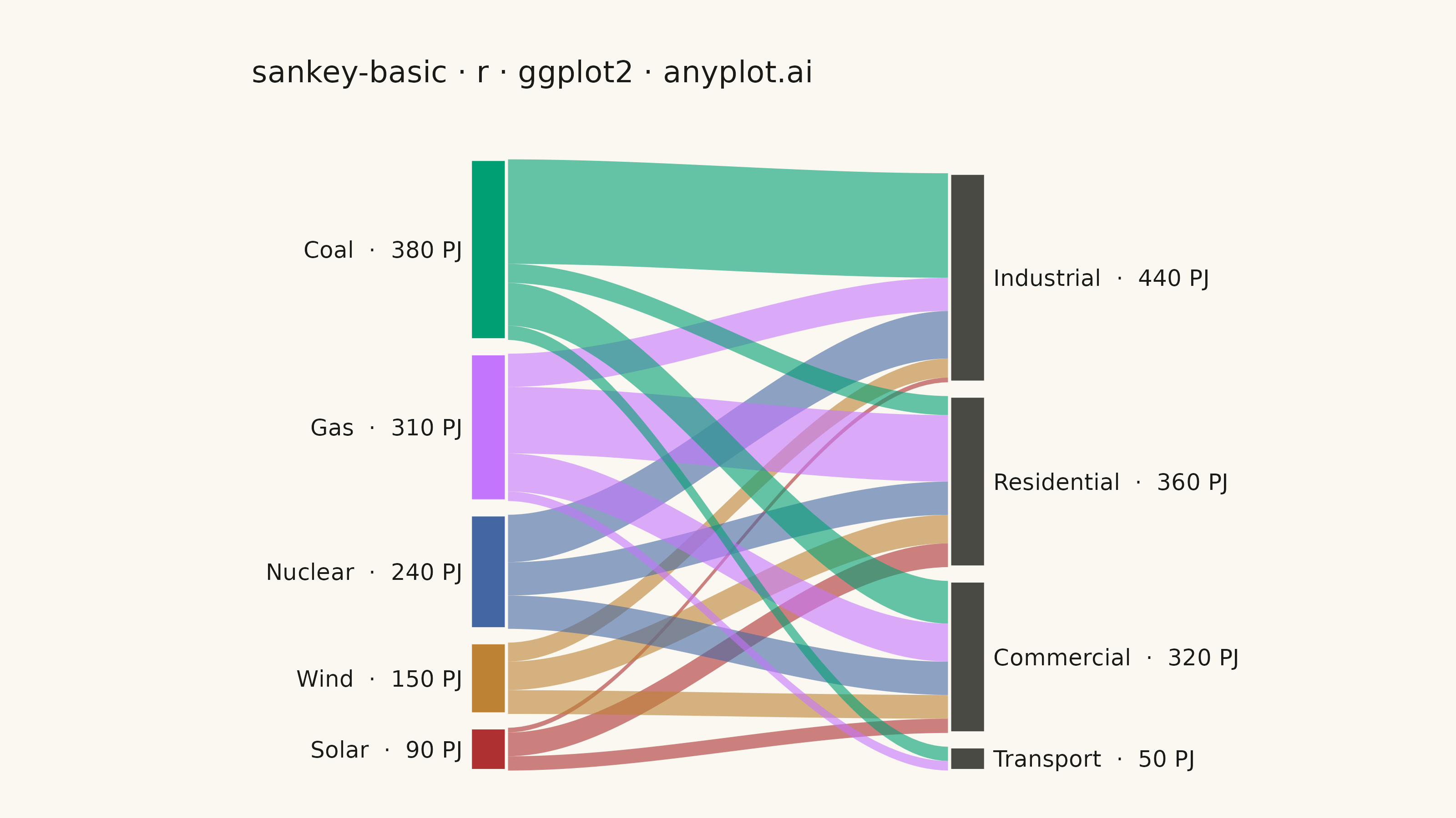
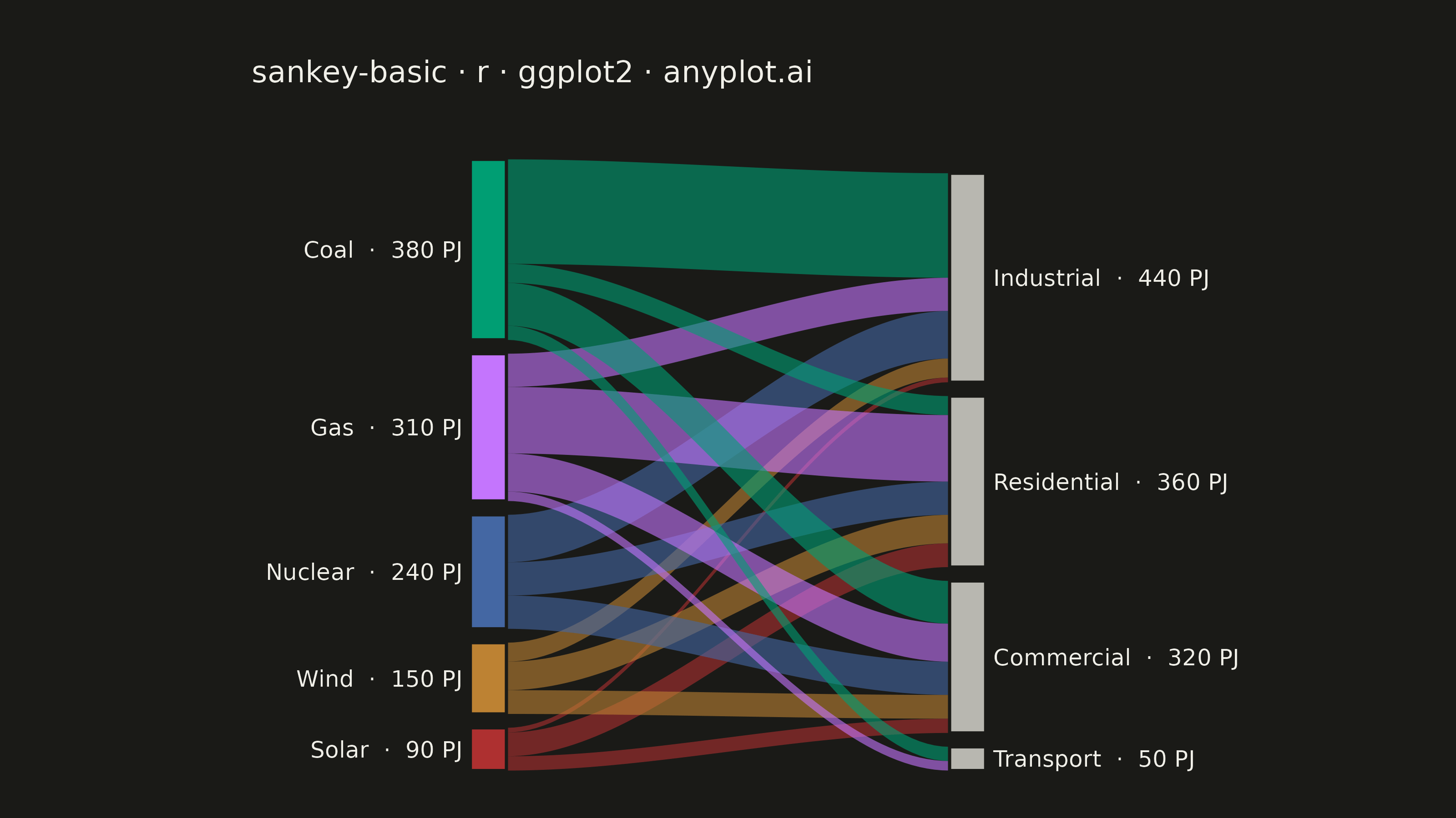
A Sankey diagram visualizes flow or transfer between nodes using links with widths proportional to flow values. It excels at showing how quantities distribute from sources to destinations, revealing patterns in resource allocation, process flows, and system transitions. The diagram makes it easy to identify major pathways and compare relative magnitudes of different flows.
#' anyplot.ai
#' sankey-basic: Basic Sankey Diagram
#' Library: ggplot2 3.5.1 | R 4.4.1
#' Quality: 93/100 | Created: 2026-07-25

library(ggplot2)
library(dplyr)
library(tidyr)
library(tibble)
library(ragg)

set.seed(42)

# --- Theme tokens -------------------------------------------------------
THEME    <- Sys.getenv("ANYPLOT_THEME", "light")
PAGE_BG  <- if (THEME == "light") "#FAF8F1" else "#1A1A17"
INK      <- if (THEME == "light") "#1A1A17" else "#F0EFE8"
INK_SOFT <- if (THEME == "light") "#4A4A44" else "#B8B7B0"
IMPRINT_PALETTE <- c("#009E73", "#C475FD", "#4467A3", "#BD8233",
                     "#AE3030", "#2ABCCD", "#954477", "#99B314")

# --- Data: national energy supply (PJ/year) by source and end-use sector -
flows <- tibble::tribble(
  ~source,   ~target,        ~value,
  "Coal",    "Industrial",   220,
  "Coal",    "Commercial",   90,
  "Coal",    "Residential",  40,
  "Coal",    "Transport",    30,
  "Gas",     "Residential",  140,
  "Gas",     "Commercial",   80,
  "Gas",     "Industrial",   70,
  "Gas",     "Transport",    20,
  "Nuclear", "Industrial",   100,
  "Nuclear", "Commercial",   70,
  "Nuclear", "Residential",  70,
  "Wind",    "Residential",  60,
  "Wind",    "Commercial",   50,
  "Wind",    "Industrial",   40,
  "Solar",   "Residential",  50,
  "Solar",   "Commercial",   30,
  "Solar",   "Industrial",   10
)

source_order <- c("Coal", "Gas", "Nuclear", "Wind", "Solar")
target_order <- c("Industrial", "Residential", "Commercial", "Transport")
dominant_link <- flows |> slice_max(value, n = 1, with_ties = FALSE)

# ggplot2 has no native Sankey geom; nodes/links are laid out by hand below
# (geom_rect for nodes, geom_ribbon with smoothstep-eased curves for links)
# using only ggplot2 + dplyr/tidyr pipelines (vectorized, no helper functions)
# — no ggalluvial/ggsankey/ggforce dependency.

# --- Layout: stack nodes top-down with a fixed padding between them -----
node_width <- 0.07
gap_frac   <- 0.025
total_value <- sum(flows$value)
gap <- gap_frac * total_value

source_totals <- flows |> group_by(source) |> summarise(total = sum(value)) |> tibble::deframe()
target_totals <- flows |> group_by(target) |> summarise(total = sum(value)) |> tibble::deframe()

node_stack <- bind_rows(
  tibble::tibble(side = "source", name = source_order, total = as.numeric(source_totals[source_order])),
  tibble::tibble(side = "target", name = target_order, total = as.numeric(target_totals[target_order]))
) |>
  group_by(side) |>
  mutate(
    cum_before   = cumsum(lag(total + gap, default = 0)),
    total_height = sum(total) + gap * (n() - 1),
    y1           = total_height - cum_before,
    y0           = y1 - total
  ) |>
  ungroup()

source_nodes <- node_stack |>
  filter(side == "source") |>
  mutate(xmin = 0, xmax = node_width,
         fill_color = IMPRINT_PALETTE[match(name, source_order)])

target_nodes <- node_stack |>
  filter(side == "target") |>
  mutate(xmin = 1 - node_width, xmax = 1, fill_color = INK_SOFT)

node_rects <- bind_rows(source_nodes, target_nodes)

# --- Assign each link a vertical slice within its source and target nodes
link_positions <- flows |>
  arrange(match(source, source_order), match(target, target_order)) |>
  group_by(source) |>
  mutate(src_cum1 = cumsum(value), src_cum0 = src_cum1 - value) |>
  ungroup() |>
  arrange(match(target, target_order), match(source, source_order)) |>
  group_by(target) |>
  mutate(tgt_cum1 = cumsum(value), tgt_cum0 = tgt_cum1 - value) |>
  ungroup() |>
  left_join(source_nodes |> select(source = name, src_top = y1), by = "source") |>
  left_join(target_nodes |> select(target = name, tgt_top = y1), by = "target") |>
  mutate(
    src_ymin = src_top - src_cum1,
    src_ymax = src_top - src_cum0,
    tgt_ymin = tgt_top - tgt_cum1,
    tgt_ymax = tgt_top - tgt_cum0,
    link_id  = row_number(),
    is_dominant = source == dominant_link$source & target == dominant_link$target
  )

dominant_id <- link_positions$link_id[link_positions$is_dominant]

# --- Interpolate every link into a smooth ribbon (cubic smoothstep ease) -
# One vectorized crossing (data x sample-points) replaces a per-row helper.
curves <- link_positions |>
  select(link_id, source, src_ymin, src_ymax, tgt_ymin, tgt_ymax) |>
  crossing(t = seq(0, 1, length.out = 60)) |>
  mutate(
    ease = t^2 * (3 - 2 * t),
    x    = node_width + (1 - 2 * node_width) * t,
    ymin = src_ymin + (tgt_ymin - src_ymin) * ease,
    ymax = src_ymax + (tgt_ymax - src_ymax) * ease
  )

curve_fill_values <- setNames(IMPRINT_PALETTE[seq_along(source_order)], source_order)

# --- Title (fontsize scales with title length, see plot-generator.md) ---
title_str <- "sankey-basic · r · ggplot2 · anyplot.ai"
title_ratio <- if (nchar(title_str) > 67) 67 / nchar(title_str) else 1.0
title_fontsize <- round(12 * title_ratio)

# --- Plot -----------------------------------------------------------------
p <- ggplot() +
  # Flat fills for every ribbon.
  geom_ribbon(
    data = curves,
    aes(x = x, ymin = ymin, ymax = ymax, group = link_id, fill = source),
    alpha = 0.55, color = NA
  ) +
  # Thin edge stroke on every ribbon keeps individual flows legible where
  # dense crossing bands would otherwise blend into a muddy overlap.
  geom_ribbon(
    data = curves,
    aes(x = x, ymin = ymin, ymax = ymax, group = link_id, color = source),
    fill = NA, alpha = 0.9, linewidth = 0.15
  ) +
  # Re-draw the single largest flow on top, more saturated and outlined in
  # ink, so the dominant Coal -> Industrial pathway reads at a glance.
  geom_ribbon(
    data = filter(curves, link_id == dominant_id),
    aes(x = x, ymin = ymin, ymax = ymax, group = link_id),
    fill = IMPRINT_PALETTE[1], color = INK, alpha = 0.88, linewidth = 0.35
  ) +
  geom_rect(
    data = node_rects,
    aes(xmin = xmin, xmax = xmax, ymin = y0, ymax = y1, fill = I(fill_color)),
    color = PAGE_BG, linewidth = 0.6
  ) +
  geom_text(
    data = source_nodes,
    aes(x = xmin - 0.015, y = (y0 + y1) / 2, label = paste0(name, "  ·  ", total, " PJ")),
    hjust = 1, size = 3.2, color = INK
  ) +
  geom_text(
    data = target_nodes,
    aes(x = xmax + 0.015, y = (y0 + y1) / 2, label = paste0(name, "  ·  ", total, " PJ")),
    hjust = 0, size = 3.2, color = INK
  ) +
  scale_fill_manual(values = curve_fill_values) +
  scale_color_manual(values = curve_fill_values) +
  scale_y_continuous(expand = expansion(mult = c(0.02, 0.05))) +
  coord_cartesian(xlim = c(-0.34, 1.34), clip = "off") +
  labs(title = title_str) +
  theme_void(base_size = 8) +
  theme(
    plot.background  = element_rect(fill = PAGE_BG, color = PAGE_BG),
    panel.background = element_rect(fill = PAGE_BG, color = NA),
    plot.title        = element_text(color = INK, size = title_fontsize,
                                      margin = margin(b = 16)),
    legend.position   = "none",
    plot.margin       = margin(t = 24, r = 100, b = 14, l = 100)
  )

# --- Save -------------------------------------------------------------------
ggsave(
  filename = sprintf("plot-%s.png", THEME),
  plot     = p,
  device   = ragg::agg_png,
  width    = 8,
  height   = 4.5,
  units    = "in",
  dpi      = 400
)
Runnable source as JSON, for any HTTP client: https://api.anyplot.ai/specs/sankey-basic/ggplot2/code. Any spec id and library id listed in llms-full.txt fit the same URL shape; every URL below is complete and callable.
{
  "spec_id": "sankey-basic",
  "language": "r",
  "library": "ggplot2",
  "page": "https://anyplot.ai/sankey-basic/r/ggplot2",
  "hub": "https://anyplot.ai/sankey-basic",
  "code_json": "https://api.anyplot.ai/specs/sankey-basic/ggplot2/code",
  "spec_json": "https://api.anyplot.ai/specs/sankey-basic",
  "render_light_png": "https://storage.googleapis.com/anyplot-images/plots/sankey-basic/r/ggplot2/plot-light.png",
  "render_dark_png": "https://storage.googleapis.com/anyplot-images/plots/sankey-basic/r/ggplot2/plot-dark.png",
  "quality_score": 93.0,
  "license": "MIT",
  "guide": "https://anyplot.ai/llms.txt"
}
Part of Basic Sankey Diagram on anyplot.ai.