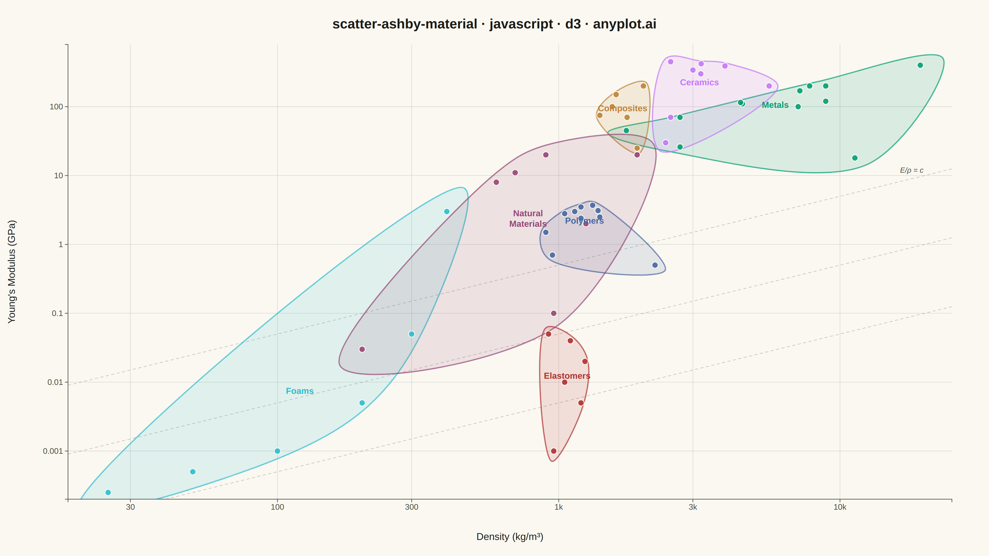
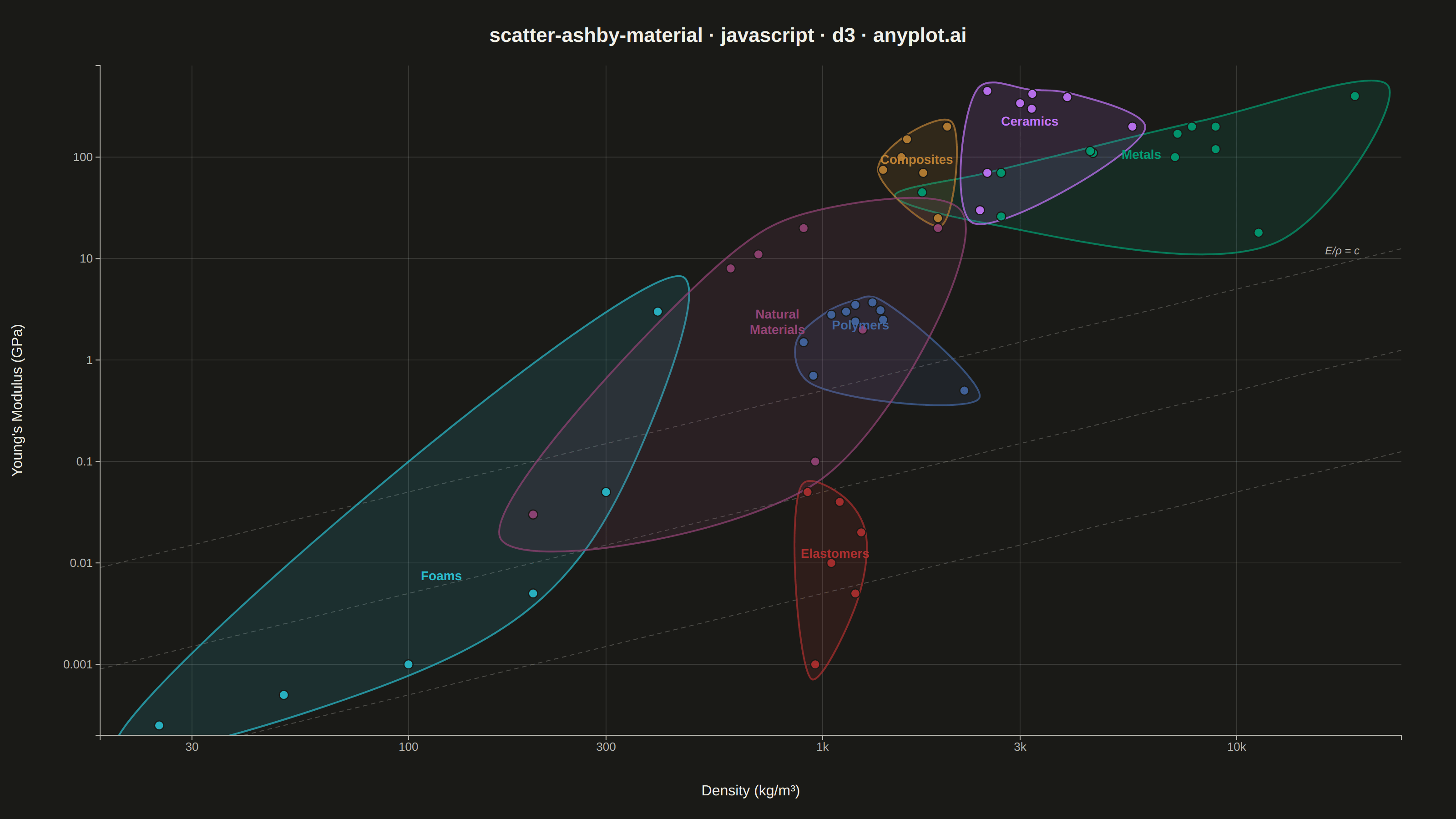
The same plot in 14 other libraries — JavaScript: Chart.js, Apache ECharts, Highcharts, MUI X Charts; Python: Altair, Bokeh, lets-plot, Matplotlib, Plotly, plotnine, Pygal, Seaborn; R: ggplot2; Julia: Makie.jl. Compare all 15 side by side: Ashby Material Selection Chart in Python, R, Julia and JavaScript.
A log-log scatter plot comparing two material properties (e.g., Young's modulus vs. density) with material families displayed as labeled bubble regions. Developed by Michael Ashby for systematic material selection in engineering design, this chart enables rapid visual comparison of material classes across multiple property dimensions. It is a standard tool in materials science and mechanical engineering education.
// anyplot.ai
// scatter-ashby-material: Ashby Material Selection Chart
// Library: d3 7.9.0 | JavaScript 22.22.3
// Quality: 91/100 | Created: 2026-06-03

//# anyplot-orientation: landscape

const t = window.ANYPLOT_TOKENS;
const { width, height } = window.ANYPLOT_SIZE;
const margin = { top: 72, right: 60, bottom: 92, left: 110 };
const iw = width - margin.left - margin.right;
const ih = height - margin.top - margin.bottom;

// Material data: density (kg/m³) vs Young's modulus (GPa)
const data = [
  // Metals
  { family: "Metals", rho: 7800,  E: 200  },
  { family: "Metals", rho: 2700,  E: 70   },
  { family: "Metals", rho: 4500,  E: 110  },
  { family: "Metals", rho: 8900,  E: 120  },
  { family: "Metals", rho: 1740,  E: 45   },
  { family: "Metals", rho: 8900,  E: 200  },
  { family: "Metals", rho: 7200,  E: 170  },
  { family: "Metals", rho: 19300, E: 400  },
  { family: "Metals", rho: 11300, E: 18   },
  { family: "Metals", rho: 7100,  E: 100  },
  { family: "Metals", rho: 4430,  E: 115  },
  { family: "Metals", rho: 2700,  E: 26   },
  // Ceramics
  { family: "Ceramics", rho: 3900, E: 390 },
  { family: "Ceramics", rho: 3210, E: 420 },
  { family: "Ceramics", rho: 2500, E: 70  },
  { family: "Ceramics", rho: 3200, E: 300 },
  { family: "Ceramics", rho: 2400, E: 30  },
  { family: "Ceramics", rho: 5600, E: 200 },
  { family: "Ceramics", rho: 2500, E: 450 },
  { family: "Ceramics", rho: 3000, E: 340 },
  // Polymers
  { family: "Polymers", rho: 1320, E: 3.7 },
  { family: "Polymers", rho: 1200, E: 2.4 },
  { family: "Polymers", rho: 1140, E: 3.0 },
  { family: "Polymers", rho: 2200, E: 0.5 },
  { family: "Polymers", rho: 950,  E: 0.7 },
  { family: "Polymers", rho: 1200, E: 3.5 },
  { family: "Polymers", rho: 900,  E: 1.5 },
  { family: "Polymers", rho: 1400, E: 2.5 },
  { family: "Polymers", rho: 1050, E: 2.8 },
  { family: "Polymers", rho: 1380, E: 3.1 },
  // Composites
  { family: "Composites", rho: 1600, E: 150 },
  { family: "Composites", rho: 1900, E: 25  },
  { family: "Composites", rho: 1400, E: 75  },
  { family: "Composites", rho: 2000, E: 200 },
  { family: "Composites", rho: 1750, E: 70  },
  { family: "Composites", rho: 1550, E: 100 },
  // Elastomers
  { family: "Elastomers", rho: 920,  E: 0.05  },
  { family: "Elastomers", rho: 1200, E: 0.005 },
  { family: "Elastomers", rho: 1100, E: 0.04  },
  { family: "Elastomers", rho: 1240, E: 0.02  },
  { family: "Elastomers", rho: 960,  E: 0.001 },
  { family: "Elastomers", rho: 1050, E: 0.01  },
  // Foams
  { family: "Foams", rho: 25,  E: 0.00025 },
  { family: "Foams", rho: 50,  E: 0.0005  },
  { family: "Foams", rho: 100, E: 0.001   },
  { family: "Foams", rho: 200, E: 0.005   },
  { family: "Foams", rho: 300, E: 0.05    },
  { family: "Foams", rho: 400, E: 3.0     },
  // Natural Materials
  { family: "Natural", rho: 200,  E: 0.03 },
  { family: "Natural", rho: 600,  E: 8    },
  { family: "Natural", rho: 700,  E: 11   },
  { family: "Natural", rho: 900,  E: 20   },
  { family: "Natural", rho: 960,  E: 0.1  },
  { family: "Natural", rho: 1250, E: 2    },
  { family: "Natural", rho: 1900, E: 20   },
];

const families = ["Metals", "Ceramics", "Polymers", "Composites", "Elastomers", "Foams", "Natural"];
const colorScale = d3.scaleOrdinal().domain(families).range(t.palette);

// Log-log scales
const x = d3.scaleLog().domain([18, 25000]).range([0, iw]);
const y = d3.scaleLog().domain([0.0002, 800]).range([ih, 0]);

// SVG
const svg = d3.select("#container").append("svg").attr("width", width).attr("height", height);
const g = svg.append("g").attr("transform", `translate(${margin.left},${margin.top})`);

// Clip path for data area
svg.append("defs").append("clipPath").attr("id", "plot-area")
  .append("rect").attr("width", iw).attr("height", ih);

// Grid lines
const xTickVals = [30, 100, 300, 1000, 3000, 10000];
const yTickVals = [0.001, 0.01, 0.1, 1, 10, 100];

g.selectAll(".xg").data(xTickVals).join("line")
  .attr("x1", d => x(d)).attr("x2", d => x(d))
  .attr("y1", 0).attr("y2", ih)
  .attr("stroke", t.grid).attr("stroke-width", 0.8);

g.selectAll(".yg").data(yTickVals).join("line")
  .attr("x1", 0).attr("x2", iw)
  .attr("y1", d => y(d)).attr("y2", d => y(d))
  .attr("stroke", t.grid).attr("stroke-width", 0.8);

// Guide lines: E/ρ = const (slope = 1 in log-log space, indicating equal specific stiffness)
const guideKs = [5e-6, 5e-5, 5e-4];
const guideGroup = g.append("g").attr("clip-path", "url(#plot-area)");
for (const k of guideKs) {
  const rhoA = 18, rhoB = 25000;
  const eA = k * rhoA, eB = k * rhoB;
  const clampA = Math.max(eA, 0.0002), clampB = Math.min(eB, 800);
  const rClampA = clampA / k, rClampB = clampB / k;
  guideGroup.append("line")
    .attr("x1", x(rClampA)).attr("y1", y(clampA))
    .attr("x2", x(rClampB)).attr("y2", y(clampB))
    .attr("stroke", t.inkSoft).attr("stroke-width", 1)
    .attr("stroke-dasharray", "5,4").attr("opacity", 0.3);
}

// Guide annotation — placed just inside right margin along the steepest guide
g.append("text")
  .attr("x", x(18000)).attr("y", y(5e-4 * 18000) - 10)
  .attr("text-anchor", "middle").attr("fill", t.inkSoft)
  .style("font-size", "12px").style("font-style", "italic")
  .text("E/ρ = c");

// Hull region drawing
function expandHull(hull, factor) {
  const cx = d3.mean(hull, p => p[0]);
  const cy = d3.mean(hull, p => p[1]);
  return hull.map(([px, py]) => [cx + (px - cx) * factor, cy + (py - cy) * factor]);
}

const blobLine = d3.line().curve(d3.curveCatmullRomClosed.alpha(0.5));
const byFamily = d3.group(data, d => d.family);
const hullGroup = g.append("g").attr("clip-path", "url(#plot-area)");

for (const [fam, pts] of byFamily) {
  const sc = pts.map(d => [x(d.rho), y(d.E)]);
  let hull = d3.polygonHull(sc);
  if (!hull) hull = sc;
  const expanded = expandHull(hull, 1.14);
  const col = colorScale(fam);
  hullGroup.append("path")
    .datum(expanded).attr("d", blobLine)
    .attr("fill", col).attr("fill-opacity", 0.13)
    .attr("stroke", col).attr("stroke-width", 2).attr("stroke-opacity", 0.7)
    .attr("stroke-linejoin", "round");
}

// Scatter points
g.append("g").attr("clip-path", "url(#plot-area)")
  .selectAll("circle").data(data).join("circle")
  .attr("cx", d => x(d.rho)).attr("cy", d => y(d.E))
  .attr("r", 5)
  .attr("fill", d => colorScale(d.family))
  .attr("fill-opacity", 0.9)
  .attr("stroke", t.pageBg).attr("stroke-width", 1.2);

// Family labels at visual centroid of each hull group
const labelLines = {
  "Natural": ["Natural", "Materials"],
};

for (const [fam, pts] of byFamily) {
  const sc = pts.map(d => [x(d.rho), y(d.E)]);
  const cx = d3.mean(sc, p => p[0]);
  const cy = d3.mean(sc, p => p[1]);
  const col = colorScale(fam);
  const lines = labelLines[fam] || [fam];
  const label = g.append("text")
    .attr("x", cx).attr("text-anchor", "middle")
    .attr("fill", col).style("font-size", "14px").style("font-weight", "700");
  lines.forEach((line, i) =>
    label.append("tspan")
      .attr("x", cx).attr("y", cy + (i - (lines.length - 1) / 2) * 17)
      .text(line)
  );
}

// Axes
const xAxis = g.append("g").attr("transform", `translate(0,${ih})`)
  .call(d3.axisBottom(x).tickValues(xTickVals)
    .tickFormat(d => d >= 1000 ? `${d / 1000}k` : String(d)).tickSize(5));
const yAxis = g.append("g")
  .call(d3.axisLeft(y).tickValues(yTickVals)
    .tickFormat(d3.format("~g")).tickSize(5));

for (const ax of [xAxis, yAxis]) {
  ax.selectAll("text").attr("fill", t.inkSoft).style("font-size", "13px");
  ax.selectAll("line").attr("stroke", t.inkSoft);
  ax.select(".domain").attr("stroke", t.inkSoft);
}

// Axis labels
g.append("text")
  .attr("x", iw / 2).attr("y", ih + 66)
  .attr("text-anchor", "middle").attr("fill", t.ink)
  .style("font-size", "16px").style("font-weight", "500")
  .text("Density  (kg/m³)");

g.append("text")
  .attr("transform", "rotate(-90)")
  .attr("x", -ih / 2).attr("y", -86)
  .attr("text-anchor", "middle").attr("fill", t.ink)
  .style("font-size", "16px").style("font-weight", "500")
  .text("Young's Modulus  (GPa)");

// Title
svg.append("text")
  .attr("x", width / 2).attr("y", 46)
  .attr("text-anchor", "middle").attr("fill", t.ink)
  .style("font-size", "22px").style("font-weight", "600")
  .text("scatter-ashby-material · javascript · d3 · anyplot.ai");
Runnable source as JSON, for any HTTP client: https://api.anyplot.ai/specs/scatter-ashby-material/d3/code. Any spec id and library id listed in llms-full.txt fit the same URL shape; every URL below is complete and callable.
{
  "spec_id": "scatter-ashby-material",
  "language": "javascript",
  "library": "d3",
  "page": "https://anyplot.ai/scatter-ashby-material/javascript/d3",
  "hub": "https://anyplot.ai/scatter-ashby-material",
  "code_json": "https://api.anyplot.ai/specs/scatter-ashby-material/d3/code",
  "spec_json": "https://api.anyplot.ai/specs/scatter-ashby-material",
  "render_light_png": "https://storage.googleapis.com/anyplot-images/plots/scatter-ashby-material/javascript/d3/plot-light.png",
  "render_dark_png": "https://storage.googleapis.com/anyplot-images/plots/scatter-ashby-material/javascript/d3/plot-dark.png",
  "interactive_light_html": "https://storage.googleapis.com/anyplot-images/plots/scatter-ashby-material/javascript/d3/plot-light.html",
  "interactive_dark_html": "https://storage.googleapis.com/anyplot-images/plots/scatter-ashby-material/javascript/d3/plot-dark.html",
  "quality_score": 91.0,
  "license": "MIT",
  "guide": "https://anyplot.ai/llms.txt"
}
Part of Ashby Material Selection Chart on anyplot.ai.