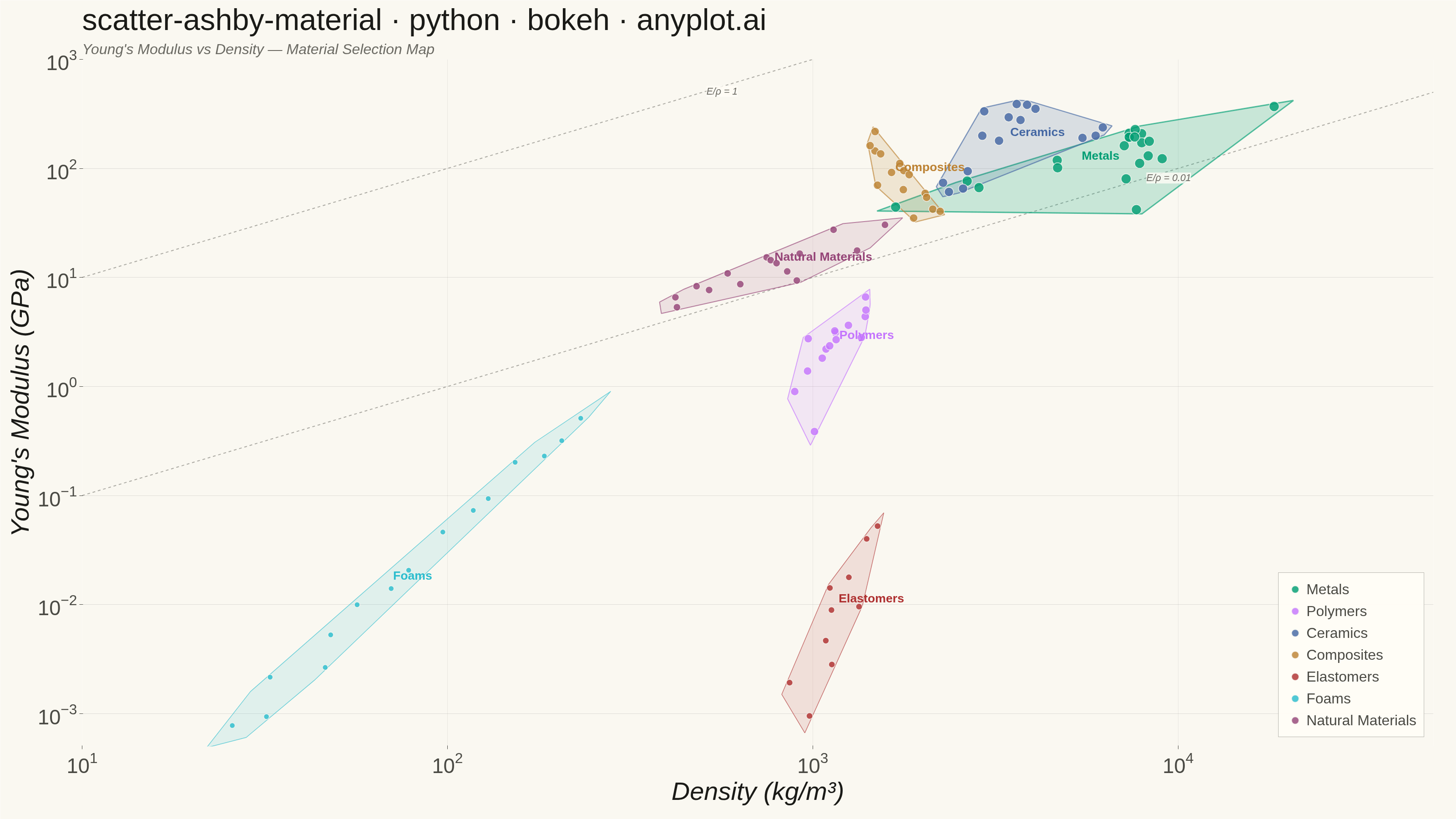
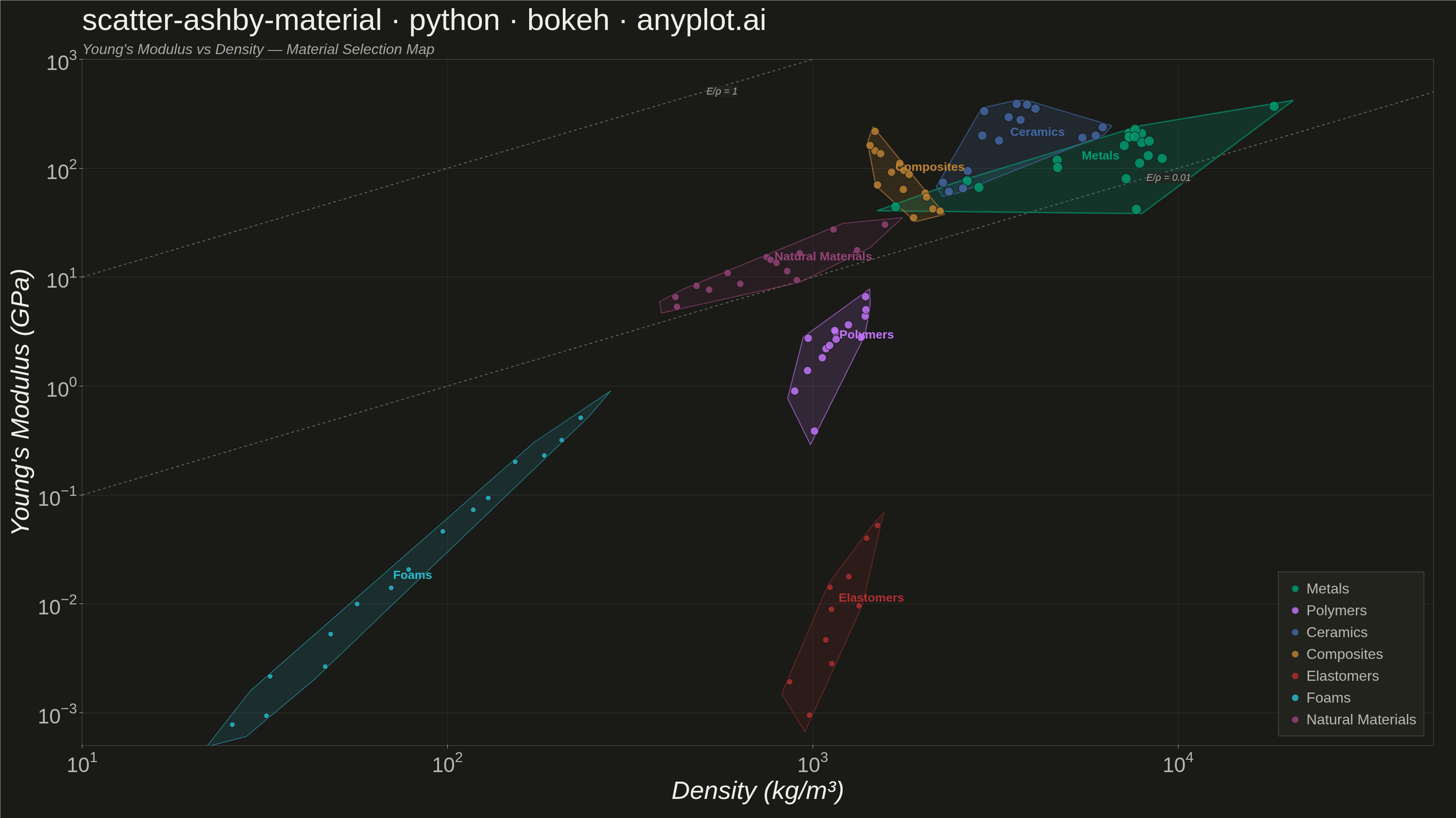
A log-log scatter plot comparing two material properties (e.g., Young's modulus vs. density) with material families displayed as labeled bubble regions. Developed by Michael Ashby for systematic material selection in engineering design, this chart enables rapid visual comparison of material classes across multiple property dimensions. It is a standard tool in materials science and mechanical engineering education.
""" anyplot.ai
scatter-ashby-material: Ashby Material Selection Chart
Library: bokeh 3.9.0 | Python 3.13.13
Quality: 90/100 | Updated: 2026-06-03
"""

import os
import sys
import time
from pathlib import Path


# Prevent this file (bokeh.py) from shadowing the bokeh package on sys.path
_here = os.path.dirname(os.path.abspath(__file__))
sys.path = [p for p in sys.path if p and os.path.abspath(p) != _here]

import numpy as np
import pandas as pd
from bokeh.io import output_file, save
from bokeh.models import ColumnDataSource, HoverTool, Label, Legend, LegendItem, Range1d, Title
from bokeh.plotting import figure
from PIL import Image
from scipy.spatial import ConvexHull
from selenium import webdriver
from selenium.webdriver.chrome.options import Options


# Theme tokens — Imprint palette style guide
THEME = os.getenv("ANYPLOT_THEME", "light")
PAGE_BG = "#FAF8F1" if THEME == "light" else "#1A1A17"
ELEVATED_BG = "#FFFDF6" if THEME == "light" else "#242420"
INK = "#1A1A17" if THEME == "light" else "#F0EFE8"
INK_SOFT = "#4A4A44" if THEME == "light" else "#B8B7B0"
INK_MUTED = "#6B6A63" if THEME == "light" else "#A8A79F"

# Imprint categorical palette — canonical order, first series always #009E73
IMPRINT_PALETTE = ["#009E73", "#C475FD", "#4467A3", "#BD8233", "#AE3030", "#2ABCCD", "#954477", "#99B314"]

# Data — density (kg/m³) vs Young's modulus (GPa) for 7 material families
np.random.seed(42)

families = {
    "Metals": {
        "density": [
            2700,
            4500,
            7800,
            7900,
            8900,
            8500,
            7300,
            19300,
            1740,
            7200,
            2800,
            7600,
            8000,
            8700,
            7100,
            4600,
            8200,
            7400,
            7850,
            8100,
        ],
        "modulus": [69, 116, 210, 193, 117, 100, 45, 400, 44, 170, 73, 200, 195, 130, 90, 110, 205, 160, 215, 180],
    },
    "Polymers": {
        "density": [950, 1050, 1200, 1400, 1140, 900, 1300, 1070, 1240, 1350, 1420, 960, 1100, 1180, 1500],
        "modulus": [0.9, 2.5, 3.0, 2.8, 3.5, 1.3, 4.0, 2.0, 2.9, 3.8, 7.0, 0.4, 1.8, 2.2, 4.5],
    },
    "Ceramics": {
        "density": [3900, 3200, 2200, 3100, 5600, 3500, 2650, 3980, 6000, 2500, 3850, 3300, 5700, 2350, 3150],
        "modulus": [380, 310, 70, 200, 210, 270, 73, 400, 230, 95, 370, 290, 200, 62, 220],
    },
    "Composites": {
        "density": [1600, 1550, 2000, 1800, 1500, 1700, 1900, 1450, 1650, 2100, 1750, 1580, 1850, 1950, 2050],
        "modulus": [140, 70, 45, 90, 180, 100, 55, 200, 120, 40, 80, 150, 65, 50, 35],
    },
    "Elastomers": {
        "density": [1100, 920, 1250, 1500, 1150, 1050, 980, 1300, 1380, 1200],
        "modulus": [0.005, 0.002, 0.01, 0.05, 0.008, 0.003, 0.001, 0.02, 0.04, 0.015],
    },
    "Foams": {
        "density": [30, 60, 120, 200, 50, 80, 150, 35, 100, 250, 45, 70, 180, 25, 110],
        "modulus": [0.001, 0.01, 0.1, 0.3, 0.005, 0.02, 0.2, 0.002, 0.05, 0.5, 0.003, 0.015, 0.25, 0.0008, 0.08],
    },
    "Natural Materials": {
        "density": [600, 700, 500, 1500, 900, 450, 800, 650, 1100, 400, 750, 550, 1300, 850, 1000],
        "modulus": [12, 14, 8, 30, 10, 6, 11, 9, 25, 5, 16, 7, 20, 13, 18],
    },
}

# Imprint palette in canonical order; 7 families use first 7 positions
family_names = list(families.keys())
family_colors = {name: IMPRINT_PALETTE[i] for i, name in enumerate(family_names)}

# Visual hierarchy — primary structural families carry more emphasis
emphasis = {
    "Metals": {"fill_alpha": 0.20, "line_width": 3.0, "marker_size": 22},
    "Ceramics": {"fill_alpha": 0.18, "line_width": 2.5, "marker_size": 20},
    "Composites": {"fill_alpha": 0.16, "line_width": 2.5, "marker_size": 18},
    "Polymers": {"fill_alpha": 0.14, "line_width": 2.0, "marker_size": 18},
    "Natural Materials": {"fill_alpha": 0.12, "line_width": 2.0, "marker_size": 16},
    "Elastomers": {"fill_alpha": 0.12, "line_width": 1.5, "marker_size": 14},
    "Foams": {"fill_alpha": 0.12, "line_width": 1.5, "marker_size": 12},
}

rows = []
for family_name, props in families.items():
    for d, m in zip(props["density"], props["modulus"], strict=True):
        jitter_d = d * (1 + np.random.uniform(-0.08, 0.08))
        jitter_m = m * (1 + np.random.uniform(-0.12, 0.12))
        rows.append({"family": family_name, "density": jitter_d, "modulus": jitter_m})
df = pd.DataFrame(rows)

# Title — 52 chars < 67 baseline, no font scaling needed
title_str = "scatter-ashby-material · python · bokeh · anyplot.ai"

# Plot — 3200×1800 landscape, log-log axes
p = figure(
    width=3200,
    height=1800,
    x_axis_type="log",
    y_axis_type="log",
    x_axis_label="Density (kg/m³)",
    y_axis_label="Young's Modulus (GPa)",
    title=title_str,
    x_range=Range1d(10, 50000),
    y_range=Range1d(0.0005, 1000),
    toolbar_location=None,
    min_border_bottom=160,
    min_border_left=180,
    min_border_top=110,
    min_border_right=50,
)

# Subtitle
p.add_layout(
    Title(
        text="Young's Modulus vs Density — Material Selection Map",
        text_font_size="24pt",
        text_color=INK_MUTED,
        text_font_style="italic",
    ),
    "above",
)

# Hover tooltip
p.add_tools(
    HoverTool(tooltips=[("Family", "@family"), ("Density", "@density{0,0} kg/m³"), ("Modulus", "@modulus{0.000} GPa")])
)

# Performance index guide lines — E/ρ = constant (slope 1 on log-log)
for c_val, label_text, lx, ly in [(0.01, "E/ρ = 0.01", 8000, 0.01 * 8000), (1.0, "E/ρ = 1", 500, 1.0 * 500)]:
    p.line(
        [10, 50000],
        [c_val * 10, c_val * 50000],
        line_color=INK_MUTED,
        line_width=2.0,
        line_dash="dashed",
        line_alpha=0.55,
    )
    p.add_layout(
        Label(
            x=lx,
            y=ly,
            text=label_text,
            text_font_size="16pt",
            text_font_style="italic",
            text_color=INK_MUTED,
            x_offset=8,
            y_offset=-10,
            background_fill_color=ELEVATED_BG,
            background_fill_alpha=0.80,
        )
    )

# Convex hull envelopes + centroid labels per family
legend_items = []
for family_name in family_names:
    fam_df = df[df["family"] == family_name]
    log_x = np.log10(fam_df["density"].values)
    log_y = np.log10(fam_df["modulus"].values)
    color = family_colors[family_name]
    emph = emphasis[family_name]

    if len(fam_df) >= 3:
        pts = np.column_stack([log_x, log_y])
        hull = ConvexHull(pts)
        hull_indices = list(hull.vertices) + [hull.vertices[0]]
        hull_pts = pts[hull_indices]

        center_log_x = pts[hull.vertices, 0].mean()
        center_log_y = pts[hull.vertices, 1].mean()

        # Tighter expand for crowded upper region, more room for sparse lower families
        expand_factor = 0.10 if family_name in ("Metals", "Ceramics", "Composites") else 0.16
        expanded = hull_pts.copy()
        for i in range(len(expanded)):
            dx = expanded[i, 0] - center_log_x
            dy = expanded[i, 1] - center_log_y
            expanded[i, 0] += dx * expand_factor
            expanded[i, 1] += dy * expand_factor

        p.patch(
            list(10 ** expanded[:, 0]),
            list(10 ** expanded[:, 1]),
            fill_alpha=emph["fill_alpha"],
            fill_color=color,
            line_color=color,
            line_alpha=0.65,
            line_width=emph["line_width"],
        )

        # Label at log-space centroid — reduces crowding vs top-of-hull approach
        p.add_layout(
            Label(
                x=10**center_log_x,
                y=10**center_log_y,
                text=family_name,
                text_font_size="20pt",
                text_font_style="bold",
                text_color=color,
                x_offset=0,
                y_offset=10,
            )
        )

# Scatter points per family
for family_name in family_names:
    fam_df = df[df["family"] == family_name]
    source = ColumnDataSource(
        data={
            "x": fam_df["density"].values,
            "y": fam_df["modulus"].values,
            "density": fam_df["density"].values,
            "modulus": fam_df["modulus"].values,
            "family": fam_df["family"].values,
        }
    )
    emph = emphasis[family_name]
    renderer = p.scatter(
        x="x",
        y="y",
        source=source,
        size=emph["marker_size"],
        color=family_colors[family_name],
        alpha=0.82,
        line_color=PAGE_BG,
        line_width=1.5,
    )
    legend_items.append(LegendItem(label=family_name, renderers=[renderer]))

# Inside legend — bottom_right is empty in this Ashby chart layout
legend = Legend(
    items=legend_items,
    location="bottom_right",
    label_text_font_size="24pt",
    label_text_color=INK_SOFT,
    glyph_height=40,
    glyph_width=40,
    spacing=8,
    padding=16,
    margin=20,
    background_fill_alpha=0.92,
    background_fill_color=ELEVATED_BG,
    border_line_color=INK_SOFT,
    border_line_alpha=0.4,
)
p.add_layout(legend)

# Typography
p.title.text_font_size = "50pt"
p.title.text_color = INK
p.title.text_font_style = "normal"

p.xaxis.axis_label_text_font_size = "42pt"
p.yaxis.axis_label_text_font_size = "42pt"
p.xaxis.axis_label_text_color = INK
p.yaxis.axis_label_text_color = INK

p.xaxis.major_label_text_font_size = "34pt"
p.yaxis.major_label_text_font_size = "34pt"
p.xaxis.major_label_text_color = INK_SOFT
p.yaxis.major_label_text_color = INK_SOFT

# Grid — both axes, subtle opacity for log-log scatter
p.xgrid.grid_line_color = INK
p.ygrid.grid_line_color = INK
p.xgrid.grid_line_alpha = 0.08
p.ygrid.grid_line_alpha = 0.12
p.xgrid.grid_line_width = 1
p.ygrid.grid_line_width = 1

# Chrome — remove outline and axis lines for a clean Ashby aesthetic
p.outline_line_color = None
p.xaxis.axis_line_color = None
p.yaxis.axis_line_color = None
p.xaxis.minor_tick_line_color = None
p.yaxis.minor_tick_line_color = None
p.xaxis.major_tick_line_color = INK_SOFT
p.yaxis.major_tick_line_color = INK_SOFT
p.background_fill_color = PAGE_BG
p.border_fill_color = PAGE_BG

# Save HTML (catalog interactive artifact)
output_file(f"plot-{THEME}.html")
save(p)

# Screenshot PNG via headless Chrome — Selenium 4 / Selenium Manager.
# Chrome's viewport is smaller than the window size by a fixed overhead (~139 px
# on this host). Use a 400 px taller window so the full 1800 px figure is visible,
# then crop the screenshot back to exactly 3200×1800.
W, H = 3200, 1800
WIN_H = H + 400  # extra headroom so the full figure fits in the viewport
opts = Options()
for arg in (
    "--headless=new",
    "--no-sandbox",
    "--disable-dev-shm-usage",
    "--disable-gpu",
    f"--window-size={W},{WIN_H}",
    "--hide-scrollbars",
):
    opts.add_argument(arg)
driver = webdriver.Chrome(options=opts)
driver.set_window_size(W, WIN_H)
driver.get(f"file://{Path(f'plot-{THEME}.html').resolve()}")
time.sleep(3)
raw_path = f"plot-{THEME}-raw.png"
driver.save_screenshot(raw_path)
driver.quit()

# Crop screenshot to exact canvas size
img = Image.open(raw_path)
img_cropped = img.crop((0, 0, W, H))
img_cropped.save(f"plot-{THEME}.png")
Path(raw_path).unlink(missing_ok=True)
Runnable source as JSON, for any HTTP client: https://api.anyplot.ai/specs/scatter-ashby-material/bokeh/code. Any spec id and library id listed in llms-full.txt fit the same URL shape; every URL below is complete and callable.
{
  "spec_id": "scatter-ashby-material",
  "language": "python",
  "library": "bokeh",
  "page": "https://anyplot.ai/scatter-ashby-material/python/bokeh",
  "hub": "https://anyplot.ai/scatter-ashby-material",
  "code_json": "https://api.anyplot.ai/specs/scatter-ashby-material/bokeh/code",
  "spec_json": "https://api.anyplot.ai/specs/scatter-ashby-material",
  "render_light_png": "https://storage.googleapis.com/anyplot-images/plots/scatter-ashby-material/python/bokeh/plot-light.png",
  "render_dark_png": "https://storage.googleapis.com/anyplot-images/plots/scatter-ashby-material/python/bokeh/plot-dark.png",
  "interactive_light_html": "https://storage.googleapis.com/anyplot-images/plots/scatter-ashby-material/python/bokeh/plot-light.html",
  "interactive_dark_html": "https://storage.googleapis.com/anyplot-images/plots/scatter-ashby-material/python/bokeh/plot-dark.html",
  "quality_score": 90.0,
  "license": "MIT",
  "guide": "https://anyplot.ai/llms.txt"
}
Part of Ashby Material Selection Chart on anyplot.ai.