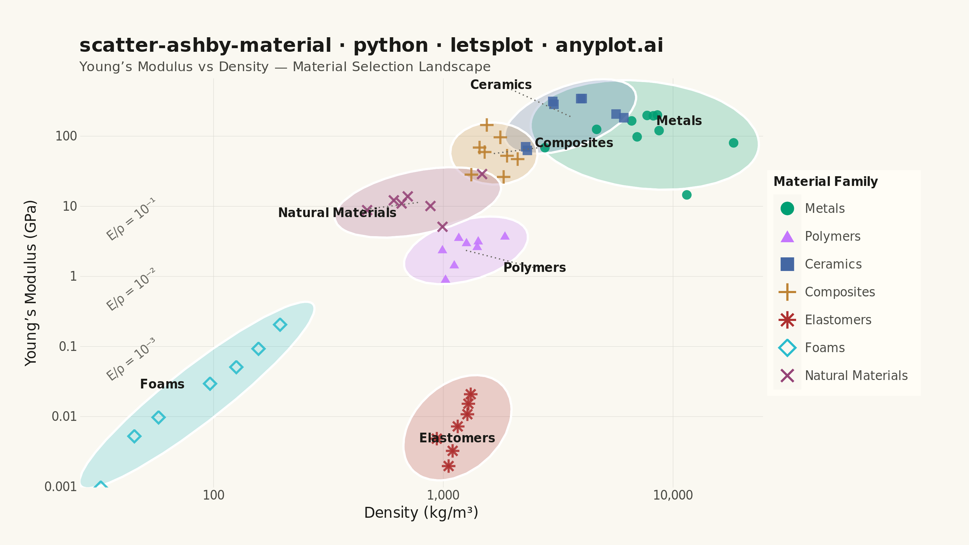
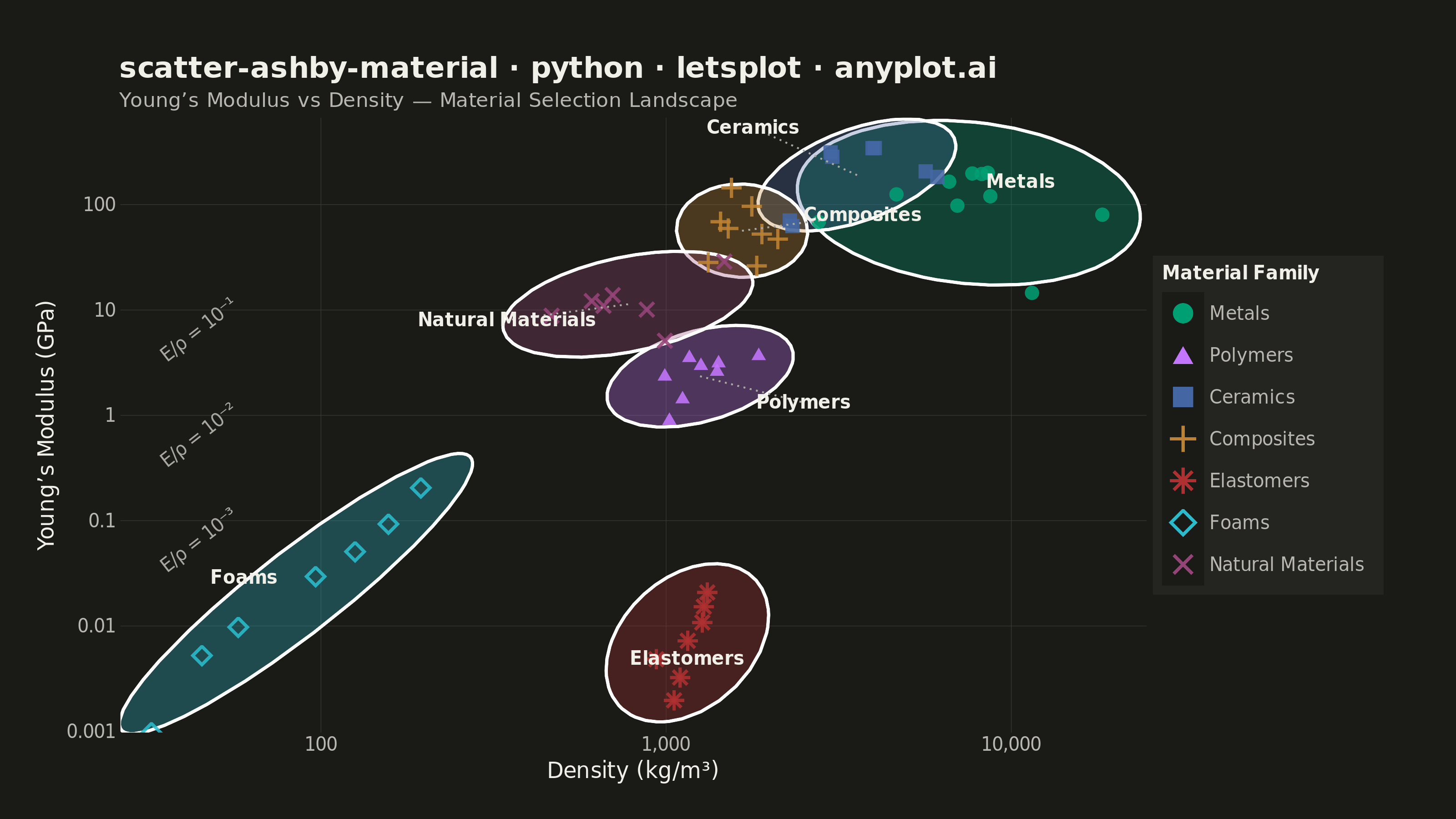
A log-log scatter plot comparing two material properties (e.g., Young's modulus vs. density) with material families displayed as labeled bubble regions. Developed by Michael Ashby for systematic material selection in engineering design, this chart enables rapid visual comparison of material classes across multiple property dimensions. It is a standard tool in materials science and mechanical engineering education.
""" anyplot.ai
scatter-ashby-material: Ashby Material Selection Chart
Library: letsplot 4.10.1 | Python 3.13.13
Quality: 86/100 | Updated: 2026-06-03
"""

import os

import numpy as np
import pandas as pd
from lets_plot import (
    LetsPlot,
    aes,
    element_blank,
    element_line,
    element_rect,
    element_text,
    geom_abline,
    geom_point,
    geom_polygon,
    geom_segment,
    geom_text,
    ggplot,
    ggsave,
    ggsize,
    guides,
    labs,
    layer_tooltips,
    scale_color_manual,
    scale_fill_manual,
    scale_shape_manual,
    scale_x_log10,
    scale_y_log10,
    theme,
    theme_minimal,
)


LetsPlot.setup_html()

# Theme tokens
THEME = os.getenv("ANYPLOT_THEME", "light")
PAGE_BG = "#FAF8F1" if THEME == "light" else "#1A1A17"
ELEVATED_BG = "#FFFDF6" if THEME == "light" else "#242420"
INK = "#1A1A17" if THEME == "light" else "#F0EFE8"
INK_SOFT = "#4A4A44" if THEME == "light" else "#B8B7B0"
INK_MUTED = "#6B6A63" if THEME == "light" else "#A8A79F"
GRID_COLOR = "#D8D7D0" if THEME == "light" else "#3A3A36"
FILL_ALPHA = 0.22 if THEME == "light" else 0.30

# Imprint palette — 7 canonical positions for 7 material families (insertion order: Metals first)
IMPRINT_7 = ["#009E73", "#C475FD", "#4467A3", "#BD8233", "#AE3030", "#2ABCCD", "#954477"]

# Data — Density (kg/m^3) vs Young's modulus (GPa) for common engineering materials
np.random.seed(42)

families = {
    "Metals": {
        "density": [2700, 4500, 7800, 7900, 8900, 8400, 11340, 7200, 19300, 7300],
        "modulus": [69, 116, 200, 193, 117, 200, 16, 170, 79, 105],
        "names": [
            "Aluminum",
            "Titanium",
            "Steel",
            "Stainless Steel",
            "Copper",
            "Nickel Alloy",
            "Lead",
            "Cast Iron",
            "Gold",
            "Tin Alloy",
        ],
    },
    "Polymers": {
        "density": [950, 1400, 1200, 1050, 1300, 1150, 1420, 1780],
        "modulus": [0.9, 2.8, 3.5, 2.3, 3.0, 1.3, 3.3, 3.9],
        "names": ["Polyethylene", "PVC", "Nylon", "Polypropylene", "PET", "Polystyrene", "Acetal", "PEEK"],
    },
    "Ceramics": {
        "density": [3980, 3200, 2200, 5680, 2500, 3100, 6000, 3900],
        "modulus": [380, 310, 70, 210, 65, 270, 200, 350],
        "names": [
            "Alumina",
            "Silicon Nitride",
            "Glass",
            "Zirconia",
            "Porcelain",
            "Silicon Carbide",
            "Tungsten Carbide",
            "Sapphire",
        ],
    },
    "Composites": {
        "density": [1600, 2000, 1500, 1800, 1550, 1400, 1700, 1900],
        "modulus": [140, 45, 70, 25, 60, 30, 90, 50],
        "names": [
            "CFRP",
            "GFRP",
            "Aramid/Epoxy",
            "Sheet Molding",
            "Carbon/PEEK",
            "Flax/Epoxy",
            "Boron/Epoxy",
            "Glass/Vinyl Ester",
        ],
    },
    "Elastomers": {
        "density": [920, 1250, 1100, 1500, 1050, 1150, 1300],
        "modulus": [0.005, 0.01, 0.003, 0.02, 0.002, 0.008, 0.015],
        "names": ["Natural Rubber", "Neoprene", "Silicone", "Fluorocarbon", "Butyl Rubber", "EPDM", "Polyurethane"],
    },
    "Foams": {
        "density": [30, 60, 120, 200, 45, 100, 160],
        "modulus": [0.001, 0.01, 0.05, 0.2, 0.005, 0.03, 0.1],
        "names": [
            "Polyurethane Foam",
            "Polystyrene Foam",
            "PVC Foam",
            "Metallic Foam",
            "PE Foam",
            "Phenolic Foam",
            "Syntactic Foam",
        ],
    },
    "Natural Materials": {
        "density": [600, 700, 500, 1500, 1000, 800, 650],
        "modulus": [12, 14, 9, 30, 5, 10, 11],
        "names": ["Oak", "Maple", "Balsa", "Bone", "Cork", "Bamboo", "Pine"],
    },
}

# Build dataframe with small scatter noise for visual spread
rows = []
for family, props in families.items():
    for d, m, name in zip(props["density"], props["modulus"], props["names"], strict=True):
        noise_d = np.exp(np.random.normal(0, 0.05))
        noise_m = np.exp(np.random.normal(0, 0.05))
        rows.append({"material": name, "family": family, "density": d * noise_d, "modulus": m * noise_m})

df = pd.DataFrame(rows)

# Elliptical envelopes per family (eigendecomposition in log space)
envelope_rows = []
n_pts = 80
theta = np.linspace(0, 2 * np.pi, n_pts, endpoint=False)
# Tighter scales for Ceramics/Composites to reduce their overlap
envelope_scales = {"Foams": 1.8, "Elastomers": 2.2, "Ceramics": 1.9, "Composites": 1.9}
default_scale = 2.4
for family in df["family"].unique():
    sub = df[df["family"] == family]
    log_x = np.log10(sub["density"].values)
    log_y = np.log10(sub["modulus"].values)
    cx, cy = log_x.mean(), log_y.mean()
    dx, dy = log_x - cx, log_y - cy
    cov = np.array([[np.mean(dx * dx), np.mean(dx * dy)], [np.mean(dx * dy), np.mean(dy * dy)]])
    eigvals, eigvecs = np.linalg.eigh(cov)
    scale = envelope_scales.get(family, default_scale)
    for t in theta:
        pt = eigvecs @ (np.sqrt(np.maximum(eigvals, 0.01)) * scale * np.array([np.cos(t), np.sin(t)]))
        envelope_rows.append({"family": family, "density": 10 ** (cx + pt[0]), "modulus": 10 ** (cy + pt[1])})

df_envelopes = pd.DataFrame(envelope_rows)

# Label positions with manual offsets to avoid crowding
label_offsets = {
    "Metals": (0.15, 0.2),
    "Ceramics": (-0.3, 0.45),
    "Composites": (0.35, 0.15),
    "Polymers": (0.3, -0.25),
    "Elastomers": (0.0, -0.15),
    "Foams": (-0.15, 0.15),
    "Natural Materials": (-0.35, -0.15),
}
label_rows = []
for family in df["family"].unique():
    sub = df[df["family"] == family]
    log_cx = np.log10(sub["density"]).mean()
    log_cy = np.log10(sub["modulus"]).mean()
    off_x, off_y = label_offsets.get(family, (0, 0))
    label_rows.append({"family": family, "density": 10 ** (log_cx + off_x), "modulus": 10 ** (log_cy + off_y)})

df_labels = pd.DataFrame(label_rows)

# Leader lines connecting displaced labels to their envelope centres
leader_rows = []
for family in df["family"].unique():
    sub = df[df["family"] == family]
    log_cx = np.log10(sub["density"]).mean()
    log_cy = np.log10(sub["modulus"]).mean()
    off_x, off_y = label_offsets.get(family, (0, 0))
    if abs(off_x) > 0.2 or abs(off_y) > 0.2:
        leader_rows.append(
            {"x": 10**log_cx, "y": 10**log_cy, "xend": 10 ** (log_cx + off_x), "yend": 10 ** (log_cy + off_y)}
        )

df_leaders = pd.DataFrame(leader_rows)

# Performance index guide line annotation positions
guide_df = pd.DataFrame(
    {"density": [35, 35, 35], "modulus": [0.035, 0.35, 3.5], "label": ["E/ρ = 10⁻³", "E/ρ = 10⁻²", "E/ρ = 10⁻¹"]}
)

title = "scatter-ashby-material · python · letsplot · anyplot.ai"

# Plot
plot = (
    ggplot()
    # Performance index guide lines (E/rho = constant, slope=1 on log-log axes)
    + geom_abline(intercept=np.log10(0.001), slope=1, color=INK_MUTED, size=0.4, linetype="dashed")
    + geom_abline(intercept=np.log10(0.01), slope=1, color=INK_MUTED, size=0.4, linetype="dashed")
    + geom_abline(intercept=np.log10(0.1), slope=1, color=INK_MUTED, size=0.4, linetype="dashed")
    # Guide line labels (same muted color, angled to follow the slope)
    + geom_text(
        data=guide_df, mapping=aes(x="density", y="modulus", label="label"), size=5, color=INK_MUTED, angle=38, hjust=0
    )
    # Elliptical envelopes per family
    + geom_polygon(data=df_envelopes, mapping=aes(x="density", y="modulus", fill="family"), alpha=FILL_ALPHA)
    # Individual material data points with interactive tooltips; shape encodes family for CVD safety
    + geom_point(
        data=df,
        mapping=aes(x="density", y="modulus", color="family", shape="family"),
        size=3.5,
        alpha=0.88,
        tooltips=layer_tooltips()
        .format("density", ".0f")
        .format("modulus", ".3g")
        .title("@material")
        .line("Family|@family")
        .line("Density|@{density} kg/m³")
        .line("Modulus|@{modulus} GPa")
        .min_width(180),
    )
    # Dotted leader lines from envelope centre to displaced labels
    + geom_segment(
        data=df_leaders,
        mapping=aes(x="x", y="y", xend="xend", yend="yend"),
        color=INK_MUTED,
        size=0.4,
        linetype="dotted",
    )
    # Bold family name labels
    + geom_text(
        data=df_labels,
        mapping=aes(x="density", y="modulus", label="family"),
        size=5,
        color=INK,
        fontface="bold",
        label_padding=0.3,
    )
    + scale_x_log10(name="Density (kg/m³)")
    + scale_y_log10(name="Young’s Modulus (GPa)")
    + scale_color_manual(values=IMPRINT_7, name="Material Family")
    + scale_fill_manual(values=IMPRINT_7)
    + scale_shape_manual(values=[16, 17, 15, 3, 8, 5, 4], name="Material Family")
    + guides(fill="none")
    + labs(title=title, subtitle="Young’s Modulus vs Density — Material Selection Landscape")
    + theme_minimal()
    + theme(
        axis_title=element_text(size=12, color=INK),
        axis_text=element_text(size=10, color=INK_SOFT),
        plot_title=element_text(size=16, face="bold", color=INK),
        plot_subtitle=element_text(size=11, color=INK_SOFT),
        plot_margin=[30, 40, 20, 20],
        plot_background=element_rect(fill=PAGE_BG, color=PAGE_BG),
        panel_background=element_rect(fill=PAGE_BG, color=PAGE_BG),
        legend_title=element_text(size=10, face="bold", color=INK),
        legend_text=element_text(size=10, color=INK_SOFT),
        panel_grid_major=element_line(size=0.25, color=GRID_COLOR),
        panel_grid_minor=element_blank(),
        legend_position="right",
        legend_background=element_rect(fill=ELEVATED_BG, color="transparent"),
        axis_line=element_line(color=INK_SOFT, size=0.3),
    )
    + ggsize(800, 450)
)

# Save
ggsave(plot, f"plot-{THEME}.png", path=".", scale=4)
ggsave(plot, f"plot-{THEME}.html", path=".")
Runnable source as JSON, for any HTTP client: https://api.anyplot.ai/specs/scatter-ashby-material/letsplot/code. Any spec id and library id listed in llms-full.txt fit the same URL shape; every URL below is complete and callable.
{
  "spec_id": "scatter-ashby-material",
  "language": "python",
  "library": "letsplot",
  "page": "https://anyplot.ai/scatter-ashby-material/python/letsplot",
  "hub": "https://anyplot.ai/scatter-ashby-material",
  "code_json": "https://api.anyplot.ai/specs/scatter-ashby-material/letsplot/code",
  "spec_json": "https://api.anyplot.ai/specs/scatter-ashby-material",
  "render_light_png": "https://storage.googleapis.com/anyplot-images/plots/scatter-ashby-material/python/letsplot/plot-light.png",
  "render_dark_png": "https://storage.googleapis.com/anyplot-images/plots/scatter-ashby-material/python/letsplot/plot-dark.png",
  "interactive_light_html": "https://storage.googleapis.com/anyplot-images/plots/scatter-ashby-material/python/letsplot/plot-light.html",
  "interactive_dark_html": "https://storage.googleapis.com/anyplot-images/plots/scatter-ashby-material/python/letsplot/plot-dark.html",
  "quality_score": 86.0,
  "license": "MIT",
  "guide": "https://anyplot.ai/llms.txt"
}
Part of Ashby Material Selection Chart on anyplot.ai.