The same plot in 14 other libraries — Python: Altair, Bokeh, lets-plot, Matplotlib, Plotly, plotnine, Pygal, Seaborn; R: ggplot2; JavaScript: Chart.js, D3.js, Apache ECharts, Highcharts, MUI X Charts. Compare all 15 side by side: Ashby Material Selection Chart in Python, R, Julia and JavaScript.
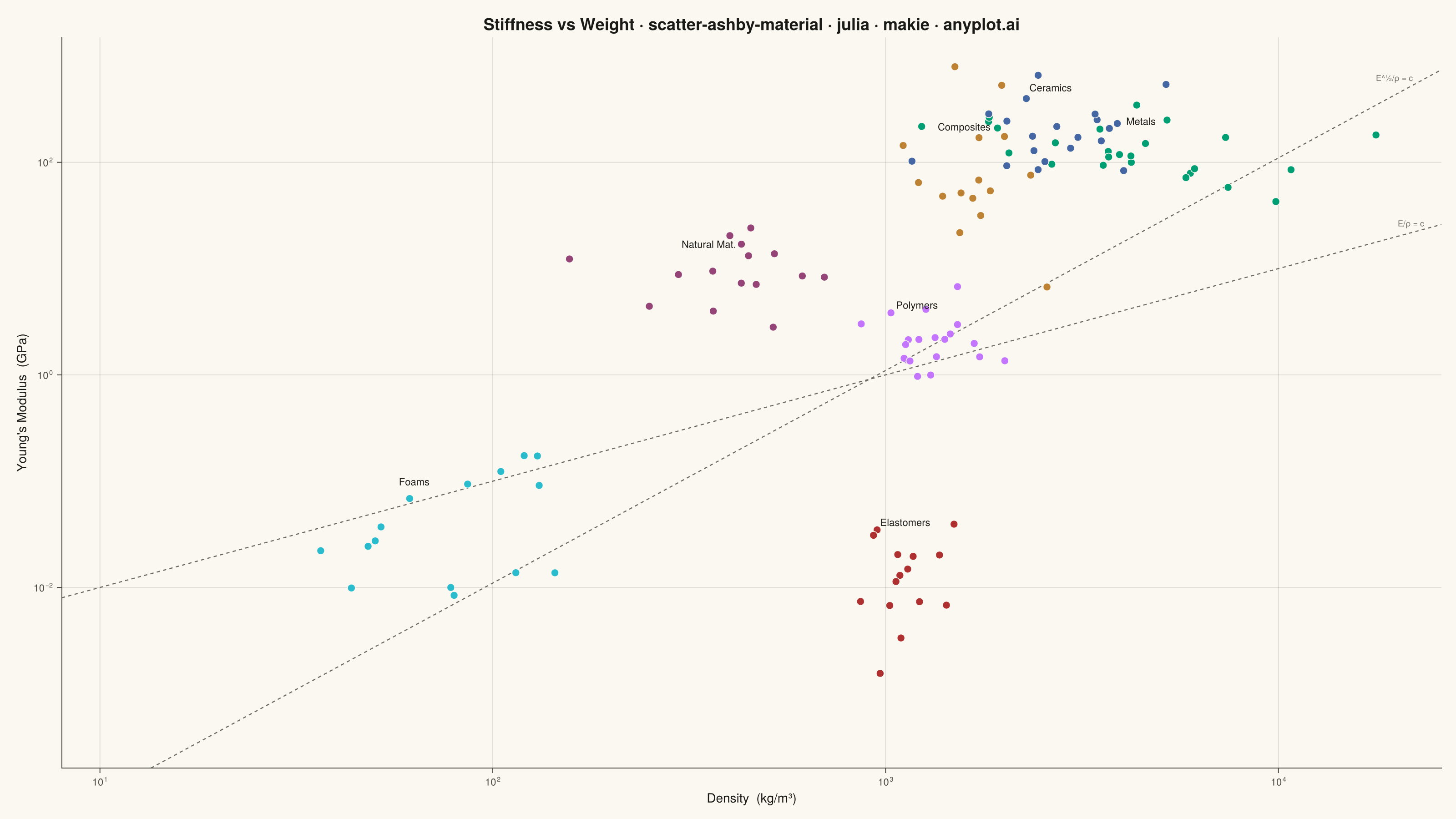
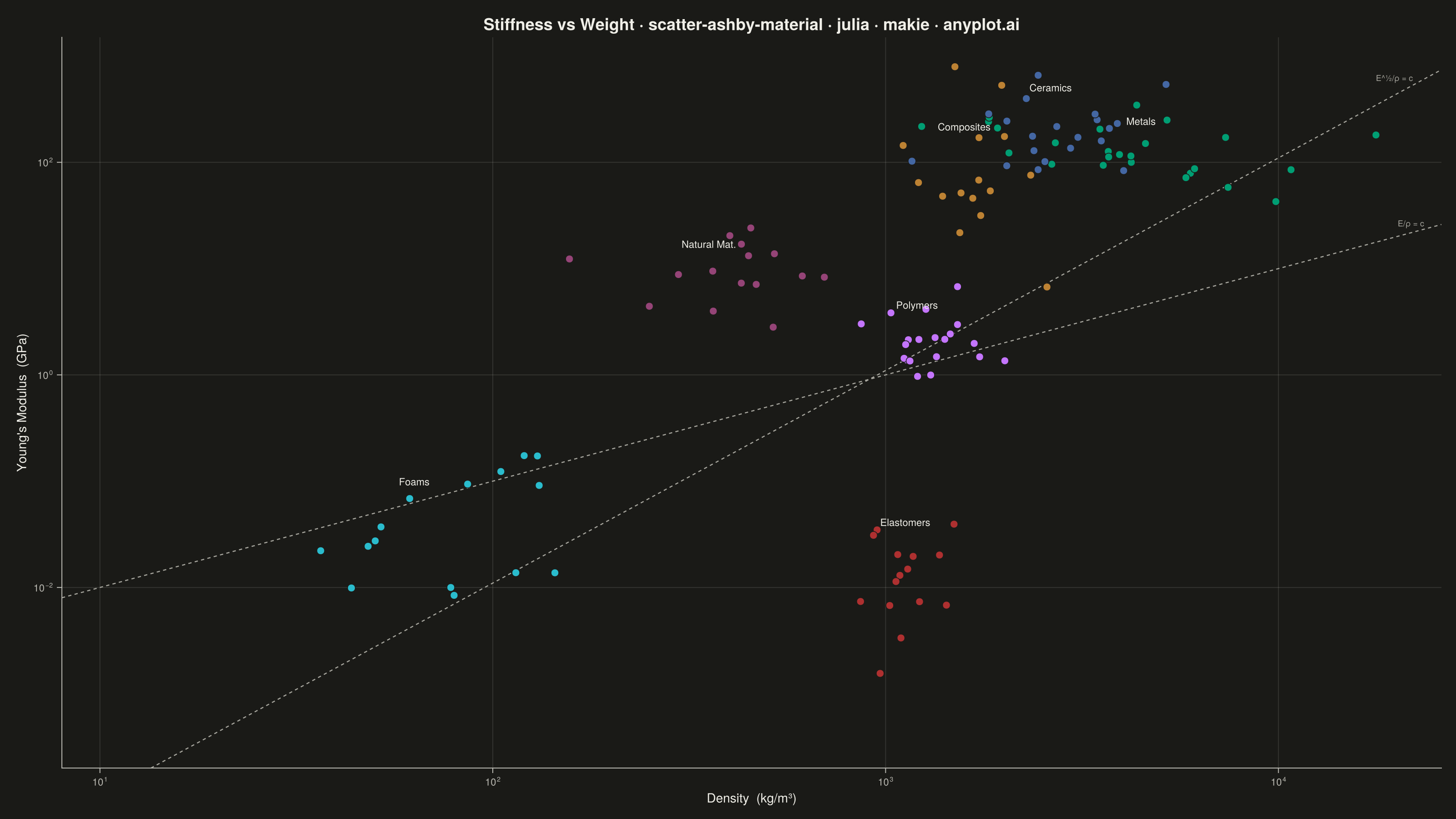
A log-log scatter plot comparing two material properties (e.g., Young's modulus vs. density) with material families displayed as labeled bubble regions. Developed by Michael Ashby for systematic material selection in engineering design, this chart enables rapid visual comparison of material classes across multiple property dimensions. It is a standard tool in materials science and mechanical engineering education.
# anyplot.ai
# scatter-ashby-material: Ashby Material Selection Chart
# Library: makie 0.22.10 | Julia 1.11.9
# Quality: 86/100 | Created: 2026-06-03

using CairoMakie
using Colors
using Random

Random.seed!(42)

# --- Theme tokens -----------------------------------------------------------
const THEME       = get(ENV, "ANYPLOT_THEME", "light")
const PAGE_BG     = THEME == "light" ? colorant"#FAF8F1" : colorant"#1A1A17"
const INK         = THEME == "light" ? colorant"#1A1A17" : colorant"#F0EFE8"
const INK_SOFT    = THEME == "light" ? colorant"#4A4A44" : colorant"#B8B7B0"
const INK_MUTED   = THEME == "light" ? colorant"#6B6A63" : colorant"#A8A79F"

const IMPRINT_PALETTE = [
    colorant"#009E73",  # 1 — brand green (Metals)
    colorant"#C475FD",  # 2 — lavender (Polymers)
    colorant"#4467A3",  # 3 — blue (Ceramics)
    colorant"#BD8233",  # 4 — ochre (Composites)
    colorant"#AE3030",  # 5 — matte red (Elastomers)
    colorant"#2ABCCD",  # 6 — cyan (Foams)
    colorant"#954477",  # 7 — rose (Natural Mat.)
]

# --- Data -------------------------------------------------------------------
# Classic density (kg/m³) vs Young's modulus (GPa) Ashby chart
# Ellipse centroid and radii defined in log10 space for accurate log-log shape
const family_names = ["Metals", "Polymers", "Ceramics", "Composites", "Elastomers", "Foams", "Natural Mat."]
const fam_cx = Float64[3.65,  3.08,  3.42,  3.20,  3.05,  1.80,  2.55]
const fam_cy = Float64[2.10,  0.30,  2.40,  1.85, -1.80, -1.50,  0.90]
const fam_rx = Float64[0.48,  0.18,  0.25,  0.16,  0.12,  0.45,  0.35]
const fam_ry = Float64[0.42,  0.55,  0.45,  0.78,  0.65,  0.80,  0.50]
const fam_n  = Int[25, 20, 20, 15, 15, 15, 15]
const n_fam  = length(family_names)

# Scatter points — generated with Gaussian noise in log space, returned in data space
all_xs = Vector{Vector{Float64}}(undef, n_fam)
all_ys = Vector{Vector{Float64}}(undef, n_fam)
for i in 1:n_fam
    all_xs[i] = 10.0 .^ (fam_cx[i] .+ randn(fam_n[i]) .* (fam_rx[i] * 0.55))
    all_ys[i] = 10.0 .^ (fam_cy[i] .+ randn(fam_n[i]) .* (fam_ry[i] * 0.55))
end

# Ellipse angle parameter (closed polygon for poly!)
const θ_pts = LinRange(0.0, 2π, 81)

# Performance index guide lines (straight lines in log-log = data-space curves)
const ρ_range  = 10.0 .^ LinRange(log10(8.0), log10(26000.0), 300)
const E_guide1 = 1.0e-3 .* ρ_range           # E/ρ = C  (slope 1, lightweight ties)
const E_guide2 = 1.1e-6 .* ρ_range .^ 2     # E^½/ρ = C (slope 2, lightweight plates)

# --- Plot -------------------------------------------------------------------
const title_str  = "Stiffness vs Weight · scatter-ashby-material · julia · makie · anyplot.ai"
const title_size = max(13, round(Int, 20 * 67 / length(title_str)))

fig = Figure(
    size            = (1600, 900),
    fontsize        = 13,
    backgroundcolor = PAGE_BG,
)

ax = Axis(
    fig[1, 1];
    title              = title_str,
    titlesize          = title_size,
    titlecolor         = INK,
    xlabel             = "Density  (kg/m³)",
    ylabel             = "Young's Modulus  (GPa)",
    xlabelsize         = 14,
    ylabelsize         = 14,
    xticklabelsize     = 11,
    yticklabelsize     = 11,
    xlabelcolor        = INK,
    ylabelcolor        = INK,
    xticklabelcolor    = INK_SOFT,
    yticklabelcolor    = INK_SOFT,
    xtickcolor         = INK_SOFT,
    ytickcolor         = INK_SOFT,
    backgroundcolor    = PAGE_BG,
    topspinevisible    = false,
    rightspinevisible  = false,
    leftspinecolor     = INK_SOFT,
    bottomspinecolor   = INK_SOFT,
    xgridcolor         = RGBAf(Float32(red(INK)), Float32(green(INK)), Float32(blue(INK)), 0.12f0),
    ygridcolor         = RGBAf(Float32(red(INK)), Float32(green(INK)), Float32(blue(INK)), 0.12f0),
    xminorgridvisible  = false,
    yminorgridvisible  = false,
    xscale             = log10,
    yscale             = log10,
)

xlims!(ax, 8.0, 26000.0)
ylims!(ax, 2.0e-4, 1500.0)

# Performance index guide lines with labels
lines!(ax, ρ_range, E_guide1;
    color     = INK_MUTED,
    linewidth = 1.2,
    linestyle = :dash,
)
lines!(ax, ρ_range, E_guide2;
    color     = INK_MUTED,
    linewidth = 1.2,
    linestyle = :dash,
)
text!(ax, 23500.0, 24.0;
    text     = "E/ρ = c",
    fontsize = 9,
    color    = INK_MUTED,
    align    = (:right, :bottom),
)
text!(ax, 22000.0, 560.0;
    text     = "E^½/ρ = c",
    fontsize = 9,
    color    = INK_MUTED,
    align    = (:right, :bottom),
)

# Material family regions, scatter points, and labels
for i in 1:n_fam
    clr = IMPRINT_PALETTE[i]

    # Ellipse polygon — defined in log space, converted to data space so Makie's
    # log10 axis transformation renders it as an ellipse in log-log view
    ell = [Point2f(10.0^(fam_cx[i] + fam_rx[i] * cos(a)),
                   10.0^(fam_cy[i] + fam_ry[i] * sin(a))) for a in θ_pts]
    poly!(ax, ell;
        color       = RGBAf(Float32(red(clr)), Float32(green(clr)), Float32(blue(clr)), 0.30f0),
        strokecolor = RGBAf(Float32(red(clr)), Float32(green(clr)), Float32(blue(clr)), 0.72f0),
        strokewidth = 1.5,
    )

    # Individual material data points
    scatter!(ax, all_xs[i], all_ys[i];
        color       = clr,
        markersize  = 12,
        strokecolor = PAGE_BG,
        strokewidth = 0.8,
    )

    # Family label offset above ellipse centroid to avoid scatter-point overlap
    text!(ax, 10.0^fam_cx[i], 10.0^(fam_cy[i] + fam_ry[i] * 0.55);
        text     = family_names[i],
        fontsize = 11,
        color    = INK,
        align    = (:center, :bottom),
    )
end

# --- Save -------------------------------------------------------------------
save("plot-$(THEME).png", fig; px_per_unit = 2)
Runnable source as JSON, for any HTTP client: https://api.anyplot.ai/specs/scatter-ashby-material/makie/code. Any spec id and library id listed in llms-full.txt fit the same URL shape; every URL below is complete and callable.
{
  "spec_id": "scatter-ashby-material",
  "language": "julia",
  "library": "makie",
  "page": "https://anyplot.ai/scatter-ashby-material/julia/makie",
  "hub": "https://anyplot.ai/scatter-ashby-material",
  "code_json": "https://api.anyplot.ai/specs/scatter-ashby-material/makie/code",
  "spec_json": "https://api.anyplot.ai/specs/scatter-ashby-material",
  "render_light_png": "https://storage.googleapis.com/anyplot-images/plots/scatter-ashby-material/julia/makie/plot-light.png",
  "render_dark_png": "https://storage.googleapis.com/anyplot-images/plots/scatter-ashby-material/julia/makie/plot-dark.png",
  "quality_score": 86.0,
  "license": "MIT",
  "guide": "https://anyplot.ai/llms.txt"
}
Part of Ashby Material Selection Chart on anyplot.ai.