The same plot in 14 other libraries — Python: Altair, Bokeh, lets-plot, Matplotlib, Plotly, plotnine, Pygal, Seaborn; Julia: Makie.jl; JavaScript: Chart.js, D3.js, Apache ECharts, Highcharts, MUI X Charts. Compare all 15 side by side: Ashby Material Selection Chart in Python, R, Julia and JavaScript.
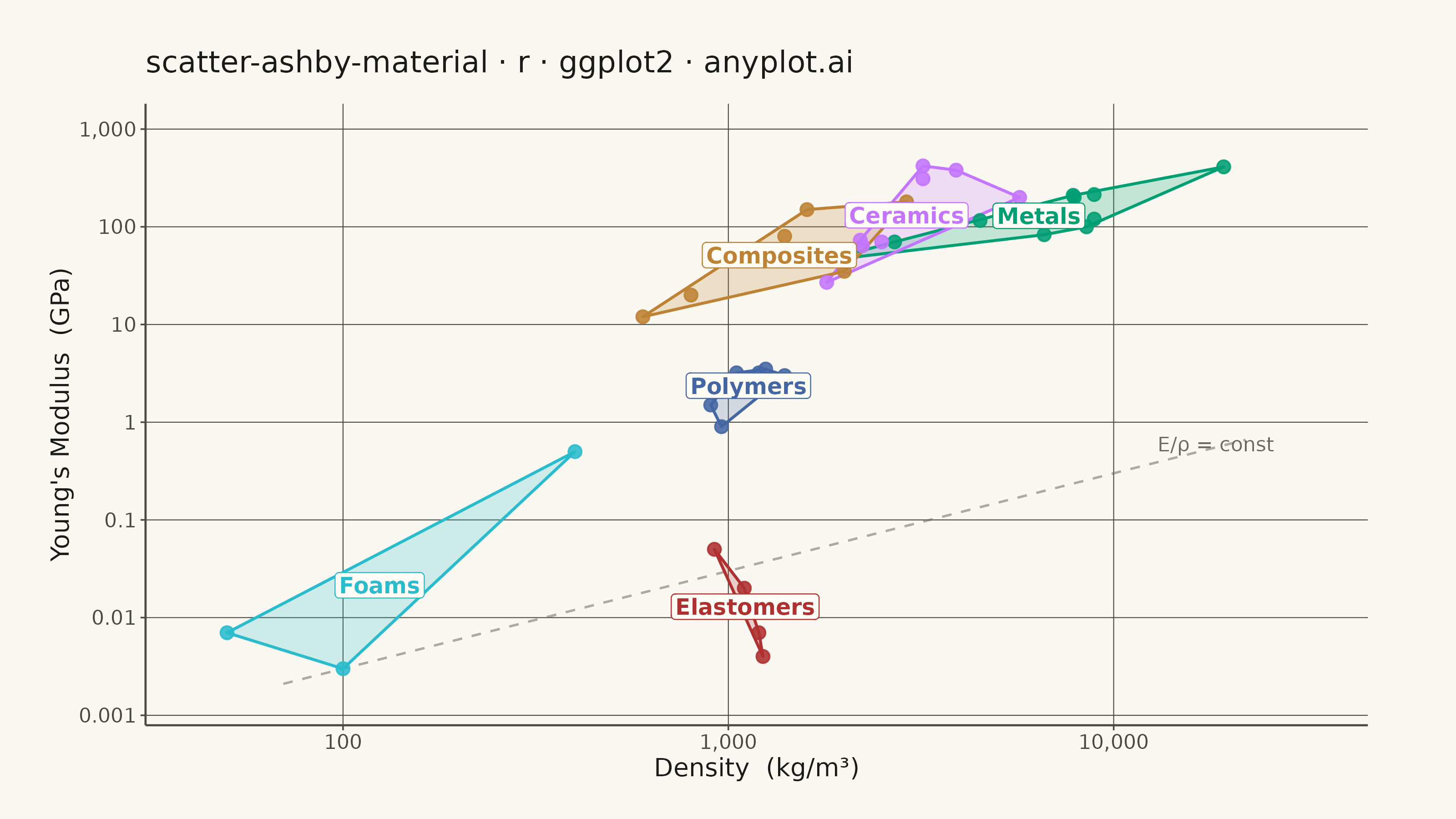
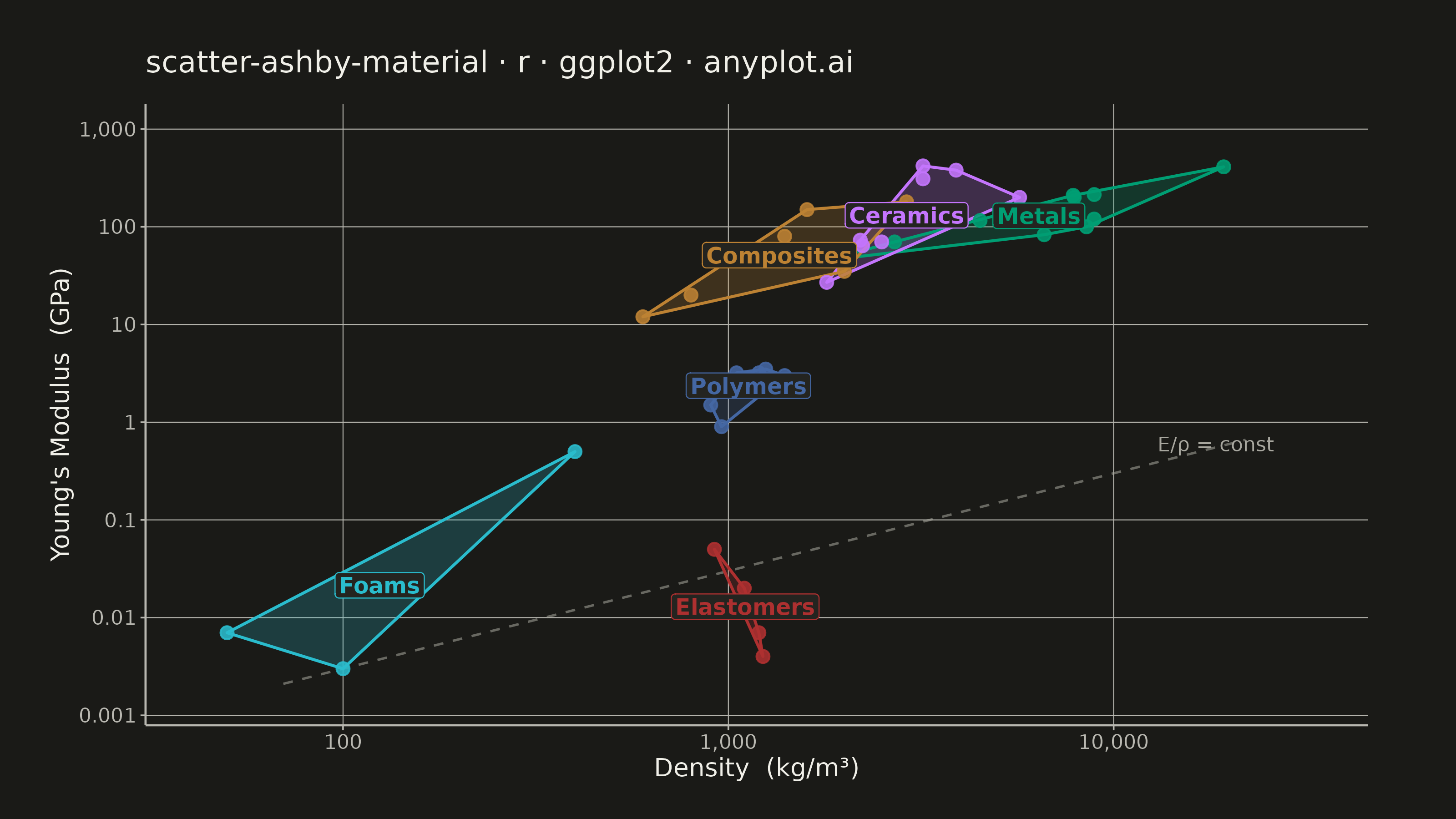
A log-log scatter plot comparing two material properties (e.g., Young's modulus vs. density) with material families displayed as labeled bubble regions. Developed by Michael Ashby for systematic material selection in engineering design, this chart enables rapid visual comparison of material classes across multiple property dimensions. It is a standard tool in materials science and mechanical engineering education.
#' anyplot.ai
#' scatter-ashby-material: Ashby Material Selection Chart
#' Library: ggplot2 3.5.1 | R 4.4.1
#' Quality: 90/100 | Created: 2026-06-03

library(ggplot2)
library(dplyr)
library(ragg)

set.seed(42)

# Theme tokens
THEME       <- Sys.getenv("ANYPLOT_THEME", "light")
PAGE_BG     <- if (THEME == "light") "#FAF8F1" else "#1A1A17"
ELEVATED_BG <- if (THEME == "light") "#FFFDF6" else "#242420"
INK         <- if (THEME == "light") "#1A1A17" else "#F0EFE8"
INK_SOFT    <- if (THEME == "light") "#4A4A44" else "#B8B7B0"
INK_MUTED   <- if (THEME == "light") "#6B6A63" else "#A8A79F"

# Imprint palette — canonical order, one color per material family
IMPRINT_PALETTE <- c(
  "#009E73",  # 1 — brand green   (Metals)
  "#C475FD",  # 2 — lavender      (Ceramics)
  "#4467A3",  # 3 — blue          (Polymers)
  "#BD8233",  # 4 — ochre         (Composites)
  "#AE3030",  # 5 — matte red     (Elastomers)
  "#2ABCCD"   # 6 — cyan          (Foams)
)

# Data: density (kg/m^3) vs Young's Modulus (GPa) — classic Ashby chart
materials <- data.frame(
  material = c(
    "Aluminum alloy", "Mild steel", "Stainless steel", "Titanium alloy",
    "Copper alloy", "Magnesium alloy", "Nickel alloy", "Tungsten",
    "Brass", "Zinc alloy",
    "Soda glass", "Borosilicate glass", "Alumina", "Silicon carbide",
    "Silicon nitride", "Zirconia", "Silica glass", "Dense graphite",
    "HDPE", "Polypropylene", "PMMA", "Nylon 66", "Epoxy resin",
    "Polystyrene", "PVC", "Polycarbonate",
    "CFRP (UD)", "GFRP", "Kevlar/epoxy", "Al/SiC composite",
    "Oak (parallel grain)", "Bamboo",
    "Natural rubber", "Silicone rubber", "Neoprene", "Polyurethane (soft)",
    "PS foam", "Rigid PU foam", "Aluminum foam", "Cork"
  ),
  family = factor(c(
    rep("Metals", 10),
    rep("Ceramics", 8),
    rep("Polymers", 8),
    rep("Composites", 6),
    rep("Elastomers", 4),
    rep("Foams", 4)
  ), levels = c("Metals", "Ceramics", "Polymers", "Composites", "Elastomers", "Foams")),
  density = c(
    2700, 7850, 7900, 4500, 8900, 1770, 8900, 19300, 8500, 6600,
    2500, 2230, 3900, 3200, 3200, 5700, 2200, 1800,
    960, 900, 1200, 1140, 1250, 1050, 1400, 1200,
    1600, 2000, 1400, 2900, 600, 800,
    920, 1200, 1230, 1100,
    50, 100, 400, 120
  ),
  modulus = c(
    70, 210, 200, 116, 120, 45, 214, 411, 100, 83,
    70, 64, 380, 420, 310, 200, 73, 27,
    0.9, 1.5, 3.2, 2.8, 3.5, 3.2, 3.0, 2.4,
    150, 35, 80, 180, 12, 20,
    0.05, 0.007, 0.004, 0.02,
    0.007, 0.003, 0.5, 0.02
  )
)

# Convex hulls computed on log-scale for accurate enclosure
hull_data <- materials %>%
  group_by(family) %>%
  slice(chull(log10(density), log10(modulus))) %>%
  ungroup()

# Label positions — geometric mean per family
label_data <- materials %>%
  group_by(family) %>%
  summarise(
    label_x = 10^mean(log10(density)),
    label_y = 10^mean(log10(modulus)),
    .groups = "drop"
  )

# Guide line: E/rho = constant (slope 1 on log-log) — lightweight stiffness direction
guide_df <- data.frame(
  density = c(70, 22000),
  modulus = c(70, 22000) * 3e-5
)

# Plot title
plot_title <- "scatter-ashby-material · r · ggplot2 · anyplot.ai"

# Build Ashby chart
p <- ggplot(materials, aes(x = density, y = modulus)) +
  # Guide line (drawn first, behind all data)
  geom_line(
    data        = guide_df,
    aes(x = density, y = modulus),
    color       = INK_MUTED,
    linewidth   = 0.45,
    linetype    = "dashed",
    alpha       = 0.55,
    inherit.aes = FALSE
  ) +
  annotate(
    "text",
    x = 13000, y = 0.6,
    label  = "E/ρ = const",
    color  = INK_MUTED,
    size   = 2.8,
    hjust  = 0,
    angle  = 0
  ) +
  # Filled convex hull regions
  geom_polygon(
    data  = hull_data,
    aes(fill = family, group = family),
    alpha = 0.22,
    color = NA
  ) +
  # Hull border outlines
  geom_polygon(
    data      = hull_data,
    aes(color = family, group = family),
    fill      = NA,
    linewidth = 0.55,
    alpha     = 0.75
  ) +
  # Individual data points
  geom_point(
    aes(color = family),
    size  = 2.1,
    alpha = 0.88
  ) +
  # Family labels inside regions
  geom_label(
    data          = label_data,
    aes(x = label_x, y = label_y, label = family, color = family),
    fill          = ELEVATED_BG,
    size          = 3.1,
    fontface      = "bold",
    label.size    = 0.2,
    label.padding = unit(0.15, "lines"),
    show.legend   = FALSE
  ) +
  scale_x_log10(
    breaks = c(100, 1000, 10000),
    labels = c("100", "1,000", "10,000"),
    expand = expansion(mult = c(0.08, 0.12))
  ) +
  scale_y_log10(
    breaks = c(0.001, 0.01, 0.1, 1, 10, 100, 1000),
    labels = c("0.001", "0.01", "0.1", "1", "10", "100", "1,000"),
    expand = expansion(mult = c(0.08, 0.12))
  ) +
  scale_color_manual(values = setNames(IMPRINT_PALETTE, levels(materials$family))) +
  scale_fill_manual(values  = setNames(IMPRINT_PALETTE, levels(materials$family))) +
  labs(
    x     = "Density  (kg/m³)",
    y     = "Young's Modulus  (GPa)",
    title = plot_title
  ) +
  theme_minimal(base_size = 8) +
  theme(
    plot.background  = element_rect(fill = PAGE_BG, color = PAGE_BG),
    panel.background = element_rect(fill = PAGE_BG, color = NA),
    panel.grid.major = element_line(color = INK_SOFT, linewidth = 0.18),
    panel.grid.minor = element_blank(),
    panel.border     = element_blank(),
    axis.title       = element_text(color = INK,      size = 10),
    axis.text        = element_text(color = INK_SOFT, size = 8),
    axis.line        = element_line(color = INK_SOFT, linewidth = 0.4),
    axis.ticks       = element_line(color = INK_SOFT, linewidth = 0.3),
    plot.title       = element_text(color = INK, size = 12,
                                    margin = margin(b = 10, unit = "pt")),
    legend.position  = "none",
    plot.margin      = margin(t = 20, r = 35, b = 15, l = 20, unit = "pt")
  )

# Save
ggsave(
  filename = sprintf("plot-%s.png", THEME),
  plot     = p,
  device   = ragg::agg_png,
  width    = 8,
  height   = 4.5,
  units    = "in",
  dpi      = 400
)
Runnable source as JSON, for any HTTP client: https://api.anyplot.ai/specs/scatter-ashby-material/ggplot2/code. Any spec id and library id listed in llms-full.txt fit the same URL shape; every URL below is complete and callable.
{
  "spec_id": "scatter-ashby-material",
  "language": "r",
  "library": "ggplot2",
  "page": "https://anyplot.ai/scatter-ashby-material/r/ggplot2",
  "hub": "https://anyplot.ai/scatter-ashby-material",
  "code_json": "https://api.anyplot.ai/specs/scatter-ashby-material/ggplot2/code",
  "spec_json": "https://api.anyplot.ai/specs/scatter-ashby-material",
  "render_light_png": "https://storage.googleapis.com/anyplot-images/plots/scatter-ashby-material/r/ggplot2/plot-light.png",
  "render_dark_png": "https://storage.googleapis.com/anyplot-images/plots/scatter-ashby-material/r/ggplot2/plot-dark.png",
  "quality_score": 90.0,
  "license": "MIT",
  "guide": "https://anyplot.ai/llms.txt"
}
Part of Ashby Material Selection Chart on anyplot.ai.